This post is based on the example discussed in Wagenmakers et al. (in press).

The Misconception

Bayes factors are a measure of absolute goodness-of-fit or absolute pre-
dictive performance.

The Correction

Bayes factors are a measure of relative goodness-of-fit or relative predictive performance. Model A may outpredict model B by a large margin, but this does not imply that model A is good, appropriate, or useful in absolute terms. In fact, model A may be absolutely terrible, just less abysmal than model B.

The Explanation

Statistical inference rarely deals in absolutes. This is widely recognized: many feel the key objective of statistical modeling is to quantify the uncertainty about parameters of interest through confidence or credible intervals. What is easily forgotten is that there is additional uncertainty, namely that which concerns the choice of the statistical model.

In other words, our statistical conclusions –including those that involve an interval estimate– are conditional on the statistical models that are employed. If these models are a poor description of reality, the resulting conclusions may be worthless at best and deeply misleading at worst.

This dictum, ‘the validity of statistical conclusions hinges on the validity of the underlying statistical models’ applies generally, but it is perhaps even more relevant for the Bayes factor, as the Bayes factor specifically compares the performance of two models.

Consider the Duke of Marlborough, who has been bludgeoned to death with a heavy candlestick. You lead the investigation and consider two suspects: the butler and the maid. You believe that both are equally likely to have committed the callous act. Then you discover that the candlestick smells of Old Spice, the butler’s favorite body spray. This is evidence that incriminates the butler and, to some extent, exonerates the maid. In other words, the presence of Old Spice on the candlestick is much more likely under the butcher-butler hypothesis than under the murderous-maid hypothesis: the Bayes factor seems to suggest that the butler is the culprit.¹ But, crucially, this conclusion depends on the fact that you entertained only two suspects, and one of them you assume is the killer. Suppose that, the next day, your forensics team finds a set of fingerprints on the candlestick, matching neither those of the butler nor those of the maid. Based on this information, you should start to doubt the absolute assertion that the butler committed the crime. The Bayes factor, however, remains unaffected — the evidence still points to the butler over the maid, to the exact same degree. Several days later, you learn that DNA found on the Duke’s body matches that of the Earl of Shropshire, who accidentally also happens to be a heavy user of Old Spice. During his arrest The Earl of Shropshire screams at the police officers: ‘the bastard had it coming, and I’m glad I did it’. In absolute terms it is clear that the butcher-butler hypothesis has become untenable. Throughout all of this, however, the Bayes factor remains exactly the same: the evidence still favors the butcher-butler hypothesis over the murderous-maid hypothesis. In the light of the Old Spice on the candlestick, the butler remains more suspect than the maid, but the fingerprints and DNA evidence make clear that the best candidate murderer was not a good candidate murderer.

An Example

The following example, paraphrased from Wagenmakers et al. (in press), was discovered purely by accident. Consider a test for a binomial rate parameter θ. The null hypothesis H₀ specifies a value of interest θ₀, and the alternative hypothesis postulates that θ is lower than θ₀, with each such value of θ deemed equally likely a priori.

A prototypical example is ‘all ravens are black’, ‘all apples grow on apple trees’, or, somewhat less traditional, ‘all zombies are hungry’. In these scenarios, H₀ represents a general law where θ₀ = 1. Consequently, the alternative hypothesis is specified as H₁ : θ ∼ Uniform[0, 1]. It is intuitively clear that the general law is destroyed upon observing a single exception: a raven that isn’t black, an apple that doesn’t grow on an apple tree, or a zombie that isn’t hungry. If we, in contrast, observe only confirmatory instances, the belief in H₀ increases. Each such instance should increase the support for the general law. The Bayes factor formalizes this intuition. For a sequence of n consecutive confirmatory instances, the Bayes factor in favor of H₀ over H₁ equals n + 1.

To make this more concrete, consider having observed 12 zombies, all of which are hungry. The results can be easily analyzed in JASP (jasp-stats.org), and the results are shown in Figure 2. Consistent with the above assertion, 12 confirmatory instances yield a Bayes factor of 13 in favor of the general law H₀ : θ₀ = 1. So far so good, but now comes a surprise.

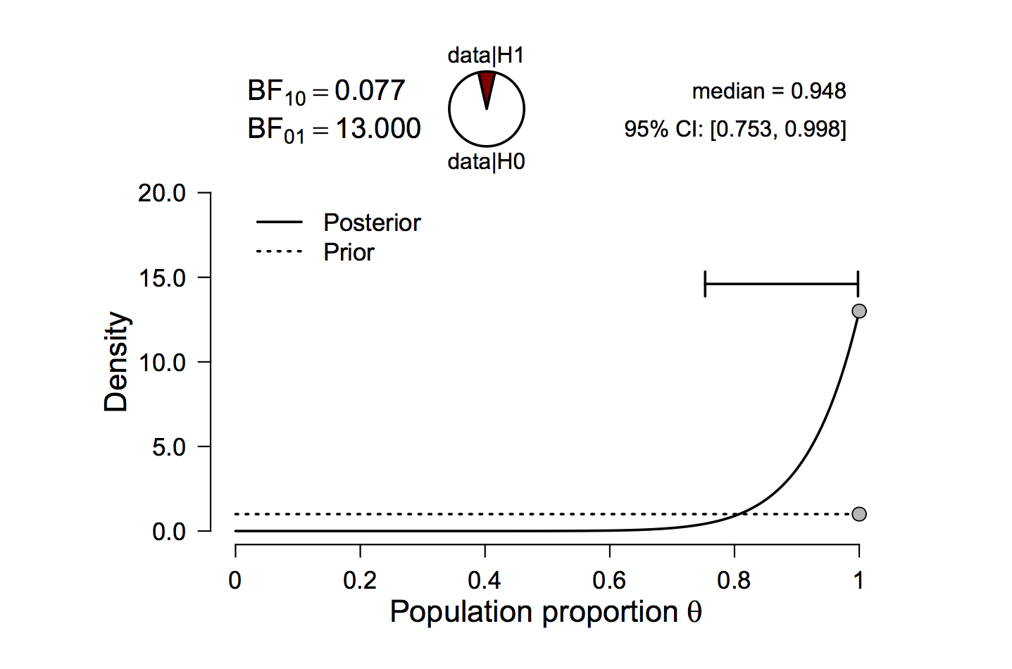
Figure 2: Twelve zombies were observed and all of them were found to be hungry. This outcome is thirteen times more likely under the general law H₀ : θ₀ = 1 than under the vague alternative H₁ : θ ∼ Uniform[0, 1]. Figure from JASP.

In 2016, we were testing the JASP implementation of the Bayesian binomial test and in the process we tried a range of different settings. One setting we tried was to retain the same data (i.e., 12 hungry zombies), but change the value of θ₀; for instance, we can choose H₀ : θ₀ = 0.25. As before, the alternative hypothesis stipulates that every value of θ smaller than θ₀ is equally likely; hence, H₁ : θ ∼ Uniform[0, 0.25]. The result is shown in Figure 3.

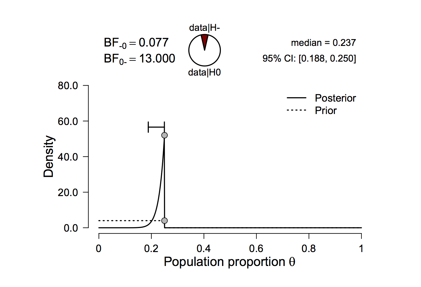
Figure 3: Twelve zombies were observed and all of them were found to be hungry. This outcome is thirteen times more likely under H₀ : θ₀ = 0.25 than under the alternative H1 : θ ∼ Uniform[0, 0.25]. Note that JASP indicates the directional nature of H1 by denoting it H_. Figure from JASP.

It turned out that the Bayes factor remains 13 in favor of H₀ over H₁, despite the fact that these two models are now defined very differently. Our initial response was that we had identified a programming mistake, but closer inspection revealed that we had stumbled upon a surprising mathematical regularity. A straightforward derivation shows that, when confronted with a series of n consecutive confirmatory instances, the Bayes factor in favor of H₀ : θ₀ = a against H₁ : θ ∼ Uniform[0, a] is always n + 1, regardless of the value for a.²

Suppose now you find yourself in a zombie apocalypse. A billion zombies are after you, and all of them appear to have a ferocious appetite. The Bayes factor for H₀ : θ₀ = a over H₁ : θ ∼ Uniform[0, a] is equal to 1,000,000,001, for any value of a, indicating overwhelming relative support in favor of H₀ over H₁. Should we therefore conclude that θ₀ = a, as stipulated by H₀? Crucially, the answer depends on the value of a. The data are perfectly consistent with H₀ : θ₀ = 1, but when θ₀ = .25 the absolute predictive performance of H₀ is abysmal. It is evident that H₀ : θ₀ = .25 provides a wholly inadequate description of reality, and placing trust in this model’s prediction would be ill-advised. What the Bayes factor shows is not that H₀ : θ₀ = .25 predicts well, but that it predicts better than H₁ : θ ∼ Uniform[0, 0.25].

Concluding Comments

It is good statistical practice to examine whether the models that are entertained provide an acceptable account of the data. When they do not, this calls into question all of the associated statistical conclusions, including those that stem from the Bayes factor. Specifically, statements such as ‘The Bayes factor supported the null hypothesis’ should be read as a convenient shorthand for the more accurate statement ‘The Bayes factor supported the null hypothesis over a particular alternative hypothesis’. In sum, the Bayes factor measures the relative predictive performance for two competing models. The model that predicts best may at the same time predict poorly.

---

 

Like this post?

Subscribe to the JASP newsletter to receive regular updates about JASP including the latest Bayesian Spectacles blog posts! You can unsubscribe at any time.

---

Footnotes

¹ Note that this interpretation as posterior odds is allowed only because both hypotheses are equally likely a priori.

² The derivation is available on the Open Science Framework. The result holds whenever θ₀ > 0.

References

Wagenmakers, E.–J., Marsman, M., Jamil, T., Ly, A., Verhagen, A. J. , Love, J., Selker, R., Gronau, Q. F., Šmíra, M., Epskamp, S., Matzke, D., Rouder, J. N., Morey, R. D. (in press). Bayesian inference for psychology. Part I: Theoretical advantages and practical ramifications. Psychonomic Bulletin & Review.

About The Authors

Eric-Jan Wagenmakers

Eric-Jan (EJ) Wagenmakers is professor at the Psychological Methods Group at the University of Amsterdam.

Quentin Gronau

Quentin is a PhD candidate at the Psychological Methods Group of the University of Amsterdam.

Wolf Vanpaemel

Wolf Vanpaemel is associate professor at the Research Group of Quantitative Psychology at the University of Leuven.