Concerns About the Default Cauchy Are Often Exaggerated: A Demonstration with JASP 0.12

May 14 - 2020

Contrary to most of the published literature, the impact of the Cauchy prior width on the t-test Bayes factor is seen to be surprisingly modest. Removing the most extreme 50% of the prior mass can at best double the Bayes factor against the null hypothesis, the same impact as conducting a one-sided instead of a two-sided test. We demonstrate this with the help of the “Equivalence T-Test” module, which was added in JASP 0.12.

We recently revised a comment on a scholarly article by Jorge Tendeiro and Henk Kiers (henceforth TK). Before getting to the main topic of this post, here is the abstract:

Tendeiro and Kiers (2019) provide a detailed and scholarly critique of Null Hypothesis Bayesian Testing (NHBT) and its central component –the Bayes factor– that allows researchers to update knowledge and quantify statistical evidence. Tendeiro and Kiers conclude that NHBT constitutes an improvement over frequentist p-values, but primarily elaborate on a list of eleven ‘issues’ of NHBT. We believe that several issues identified by Tendeiro and Kiers are of central importance for elucidating the complementary roles of hypothesis testing versus parameter estimation and for appreciating the virtue of statistical thinking over conducting statistical rituals. But although we agree with many of their thoughtful recommendations, we believe that Tendeiro and Kiers are overly pessimistic, and that several of their ‘issues’ with NHBT may in fact be conceived as pronounced advantages. We illustrate our arguments with simple, concrete examples and end with a critical discussion of one of the recommendations by Tendeiro and Kiers, which is that “estimation of the full posterior distribution offers a more complete picture” than a Bayes factor hypothesis test.

In section 3, “Use of default Bayes factors”, we address the common critique that the default Cauchy distribution (on effect size for a t-test) is so wide that the results are meaningless:

(…) in our experience the adoption of reasonable non-default prior distributions has only a modest impact on the Bayes factor (e.g., Gronau, Ly, & Wagenmakers, 2020). This impact is typically much smaller than that caused by a change in the statistical model, by variable transformations, by different treatment of outliers, and so forth. To explain why the impact of prior distributions is often surprisingly modest, consider TK’s critique that the default prior for the t-test –a Cauchy distribution centered at zero with scale parameter .707– is too wide. Specifically, this distribution assigns 50% of its mass to values larger than |.707|: if this is unrealistically wide, maybe the default prior distribution is of limited use, and the resulting Bayes factor misleading? Indeed, we ourselves have been worried in the past that the default Cauchy distribution is too wide, despite literature reviews showing that large effect sizes occur more often than one may expect (e.g., Aczel, 2018, slide 20; Wagenmakers, Wetzels, Borsboom, Kievit, & van der Maas, 2013). However, we recently realized that the impact of the ‘wideness’ is much more modest than one may intuit.

Consider two researchers, A and B, who analyze the same data set. Researcher A uses the default zero-centered Cauchy prior distribution with interquartile range of .707; researcher B uses the same prior distribution, but truncated to have mass only within the interval from −.707 to +.707. Assume that, in a very large sample, the observed effect is relatively close to zero. Researcher A reports a Bayes factor of 3.5 against the null hypothesis. It is now clear that the truncated default prior used by researcher B will provide better predictive performance, because no prior mass is ‘wasted’ on large values of effect size that are inconsistent with the data. As it turns out, truncating the default Cauchy to its interquartile range increases the predictive performance of the alternative hypothesis by a factor of at most 2. This means that the Bayes factor for B’s truncated alternative hypothesis versus A’s default ‘overly wide’ alternative hypothesis is at most 2; consequently, B will report a Bayes factor against the null hypothesis that cannot be any larger than 2 × 3.5 = 7. This means that the potential predictive benefit of truncating the default distribution to its interquartile range is just as large as the potential predictive benefit of conducting a one-sided test instead of a two-sided test.5 In other words, suppose a very large data set has an effect size of 0.3 with almost all posterior mass ranging from 0.2 to 0.4; the predictive benefit of knowing in advance the direction of the effect is just as large as the predictive benefit of knowing in advance that it falls within the prior interquartile range; consequently, the Bayes factor from a one-sided default Cauchy distribution is virtually identical to the Bayes factor from a two-sided default Cauchy distribution that is truncated to the [−.707,+.707] interval.

A Demonstration with JASP

We now provide a concrete demonstration using the “Equivalence T-Test” module from JASP 0.12. We open JASP, and from the Data Library, in the category “T-tests”, select the “Kitchen Roll” data. In Descriptives, we plot the data for “mean_NEO” across the two conditions given by “Rotation”:

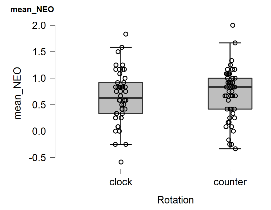
There does not appear to be a large effect here. An independent-samples Bayesian t-test with a default two-sided Cauchy prior on effect size yields the following result:

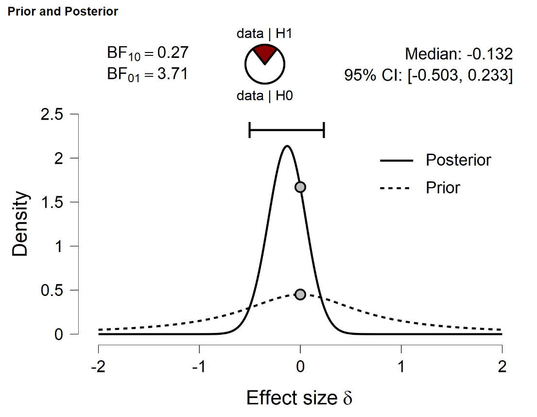
The results show that 95% of the posterior mass under H1 falls in the interval from -0.503 to 0.233, well inside the default Cauchy’s interquartile range (i.e., [−.707,+.707]). So these data are suitable to test our claim that truncating the default Cauchy to its interquartile range will give a predictive benefit that is at most 2. In other words, the Bayes factor for the truncated alternative hypothesis versus the default untruncated alternative hypothesis is at most 2. Note that this involves an overlapping hypothesis test: the truncated hypothesis is a restricted case of the untruncated hypothesis. This means that the only reason that the truncated hypothesis can predict the data better is because it is more parsimonious than the untruncated hypothesis.

To confirm this, click on the large + sign on the top right of the JASP screen to view all modules, and activate the “Equivalence T-Test” module. From the module, select the Bayesian Independent Samples T-test; drag mean_NEO to the “Variables” field and drag Rotation to the “Grouping variables” field. Then define the “Equivalence region” to range from −.707 to .707 and tick “Prior and posterior mass”. These are the resulting output tables:

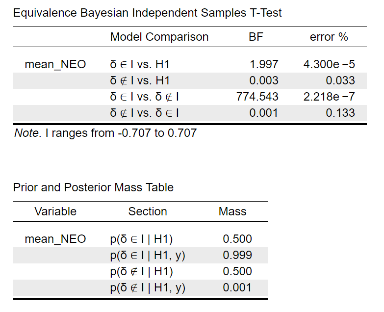
The second table confirms that almost all posterior mass (i.e., 99.9%) falls inside the specified interval (defined as the interquartile range of the default Cauchy). The first row of the first table gives the Bayes factor for the hypothesis that the effect falls inside of the interval (i.e., the truncated hypothesis) versus the hypothesis that the effect could fall anywhere (i.e., the untruncated hypothesis). The Bayes factor for this overlapping hypothesis test is 1.997 — close to its theoretical upper bound of 2.

Although not of immediate interest here, one may also consider a non-overlapping hypothesis test, one that compares the hypothesis that the effect falls inside of the interval against the hypothesis that the effect falls outside of the interval. The third row of the first table above shows that the associated Bayes factor is about 775, that is, the observed data are 775 times more likely to occur under the hypothesis that the effect falls inside of the specified interval than under the hypothesis that the effect falls outside of that interval. This highlights that different questions may evoke dramatically different answers; here, the question “it is inside of the interval instead of anywhere?” yields a BF of almost 2, whereas the question “is it inside of the interval or outside of the interval?” yields a BF of about 775. The reason for the discrepancy is that the hypothesis “it is anywhere” can actually account very well for an effect size inside the interval, whereas this is impossible for the more risky hypothesis “it is outside of the interval”.

Note that the Bayesian equivalence test demonstrated here is based on the work by Morey & Rouder (2011) and more generally on the work by Herbert Hoijtink, Irene Klugkist, and associates (e.g., Hoijtink, 2011; Hoijtink, Klugkist, & Boelen, 2008).

References

Hoijtink, H. (2011). Informative hypotheses: Theory and practice for behavioral and social scientists. Boca Raton, FL: Chapman & Hall/CRC.

Hoijtink, H., Klugkist, I., & Boelen, P. (2008) (Eds). Bayesian evaluation of informative hypotheses. New York: Springer.

Morey, R. D., & Rouder, J. N. (2011). Bayes factor approaches for testing interval null hypotheses. Psychological Methods, 16, 406-419.

van Ravenzwaaij, D., & Wagenmakers, E.-J. (2020). Advantages masquerading as ‘issues’ in Bayesian hypothesis testing: A commentary on Tendeiro and Kiers (2019). Manuscript submitted for publication.

Tendeiro, J. N., & Kiers, H. A. L. (in press). A review of issues about Null Hypothesis Bayesian Testing. Psychological Methods.

About The Authors

Eric-Jan Wagenmakers

Eric-Jan (EJ) Wagenmakers is professor at the Psychological Methods Group at the University of Amsterdam.

Don van Ravenzwaaij

Don van Ravenzwaaij (website) is an Associate Professor at the University of Groningen. In May 2018, he was awarded an NWO Vidi grant (a 5-year fellowship) for improving the evaluation of statistical evidence in the field of biomedicine. The first pillar of his research is about proper use of statistical inference in science. The second pillar is about the advancement and application of response time models to speeded decision making.