Prediction is Easy, Especially About the Past: A Critique of Posterior Bayes Factors

January 24 - 2019

The Misconception

Posterior Bayes factors are a good idea: they provide a measure of evidence but are relatively unaffected by the shape of the prior distribution.

The Correction

Posterior Bayes factors use the data twice, effectively biasing the outcome in favor of the more complex model.

The Explanation

The standard Bayes factor is the ratio of predictive performance between two rival models. For each model $M_i$ , its predictive performance $p(y | M_i)$ is computed as the likelihood for the observed data, averaged over the prior distribution for the model parameters $\theta | M_i$ . Suppressing the dependence on the model, this yields $p(y) = \int p(y | \theta) p(\theta) \, \text{d}\theta$ . Note that, as the words imply, “predictions” are generated from the “prior”. The consequence, of course, is that the shape of the prior distribution influences the predictions, and thereby the Bayes factor. Some consider this prior dependence to be a severe limitation; indeed, it would be more convenient if the observed data could be used to assist the models in making predictions — after all, it is easier to make “predictions” about the past than about the future.

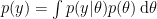
The wish to produce predictions without opening oneself up to the unwanted impact of the prior distribution has spawned an alternative to the standard Bayes factor, one in which predictions are obtained not from the prior distribution, but from the posterior distribution. This “postdictive” performance is then given by averaging the likelihood over the posterior, yielding $p^\star(y) = \int p(y | \theta) p(\theta | y) \, \text{d}\theta$ . This procedure was proposed by Aitkin (1991). Several discussants of the Aitkin paper pointed out that the method uses the data twice, inviting inferential absurdities. To see the double use of the data, note that the posterior distribution $p(\theta | y)$ is proportional to $p(y | \theta) p(\theta)$ , such that the likelihood $p(y | \theta)$ enters the formula twice.

As the rebuttal shows, Aitkin was not impressed, neither by the general argument nor by the concrete examples. Here we provide another example of posterior Bayes factors in action. Consider a binomial problem where $\mathcal{H}_0$ indicates a general law (“all apples grow on apple trees”; “all electrically neutral atoms have an equal number of protons and electrons”; “all zombies are hungry”; “all ravens are black”; “all even integers greater than two are the sum of two prime numbers”). Hence, $\mathcal{H}_0: \theta = 1$ . Our alternative model relaxes the restriction that $\theta=1$ and assigns it a prior distribution; for mathematical convenience, here we use a uniform prior from 0 to 1, that is, $\mathcal{H}_1: \theta \sim \text{beta}(a=1,b=1)$ . Furthermore, assume we only encounter confirmatory instances, that is, observations consistent with $\mathcal{H}_0$ . In this situation, every confirmatory instance ought to increase our confidence in the general law $\mathcal{H}_0$ , something that Polya (1954, p.4) called “the fundamental inductive pattern”. As we will demonstrate below, posterior Bayes factors violate the fundamental pattern (for a discussion on how Bayesian leave-one-out cross-validation or LOO also violates the fundamental pattern see Gronau & Wagenmakers, in press a, b).

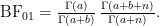
Consider first the general expression for the Bayes factor in favor of $\mathcal{H}_0: \theta = \theta_0$ over $\mathcal{H}_1: \theta \sim \text{beta}(a,b)$ :

$\text{BF}_{01} = \frac{\Gamma(a) \Gamma(b)}{\Gamma(a+b)} \thinspace \frac{\Gamma(a+b+n)}{\Gamma(a+s) \Gamma(b+f)} \thinspace \theta_0^s \thinspace (1-\theta_0)^f,$

where $s$ is the number of successes, $f$ , the number of failures, $n=s+f$ the number of attempts, and $\Gamma$ the gamma function, which for integers reduces to the factorial function: $\Gamma(x) = (x-1)!$

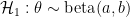
We then simplify this equation by inserting the following information: (1) $\theta_0 = 1$ (from the definition of $\mathcal{H}_0$ as a general law; (2) $f=0$ , so $n=s$ , because only successes are observed. This leaves:

$\text{BF}_{01} = \frac{\Gamma(a)}{\Gamma(a+b)} \thinspace \frac{\Gamma(a+b+n)}{\Gamma(a+n)}.$

If we assume that $a=b=1$ (the uniform prior for $\theta$ under $\mathcal{H}_1$ ) we obtain $BF_{01} = n+1$ : that is, every time a confirmatory instance is observed, the Bayes factor in favor of the general law increases by one. Thus, the standard Bayes factor generates the fundamental inductive pattern. In order to examine what the posterior Bayes factor produces, note that a $\text{beta}(a,b)$ prior distribution combined with $n=s$ successes yields a $\text{beta}(a+n, b)$ posterior distribution. This means that, under the starting assumption that $\mathcal{H}_1: \theta \sim \text{beta}(1,1)$ we can use the general equation by plugging in the posterior $\text{beta}(n+1,1)$ instead of the prior $\text{beta}(1,1)$ . Doing so yields $BF^{\star}_{01} = \frac{2n + 1}{n+1}$ .

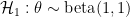
Table 1 below shows the results for various numbers of confirmatory instances $n$ . It is clear that the evidence in favor of the general law remains weak no matter how many confirmatory instances are observed. Indeed, an infinite number of confirmatory instances results in a Bayes factor of only 2;¹ if $\mathcal{H}_0$ and $\mathcal{H}_1$ are deemed equally plausible a priori, an infinite number of observations perfectly predicted by $\mathcal{H}_0$ manages to raise the probability of the general law from $.50$ to an unimpressive $.67$ . Not only this; the increase in confidence from observing a meagre 5 confirmatory instances to observing an infinite number only brings the posterior Bayes factor from about 1.83 to 2; under equal prior odds, this means that an infinite amount of confirmatory information from n=6 onwards takes the posterior probability for the general law from $0.65$ to $0.67$ , for a miniscule 2% increase.

No. confirmations $n$	$BF^{\star}_{01}$
1	$3/2 = 1.5$
2	$5/3 \approx 1.67$
3	$7/4 = 1.75$
4	$9/5 = 1.8$
5	$11/6 \approx 1.83$
$\infty$	2

Table 1. As the number of confirmatory instances $n$ increases, the posterior Bayes factor $BF^{\star}_{01}$ provides weak and bounded support for the binomial general law $\mathcal{H}_0: \theta = 1$ over the alternative model $\mathcal{H}_1: \theta \sim \text{beta}(1,1)$ .

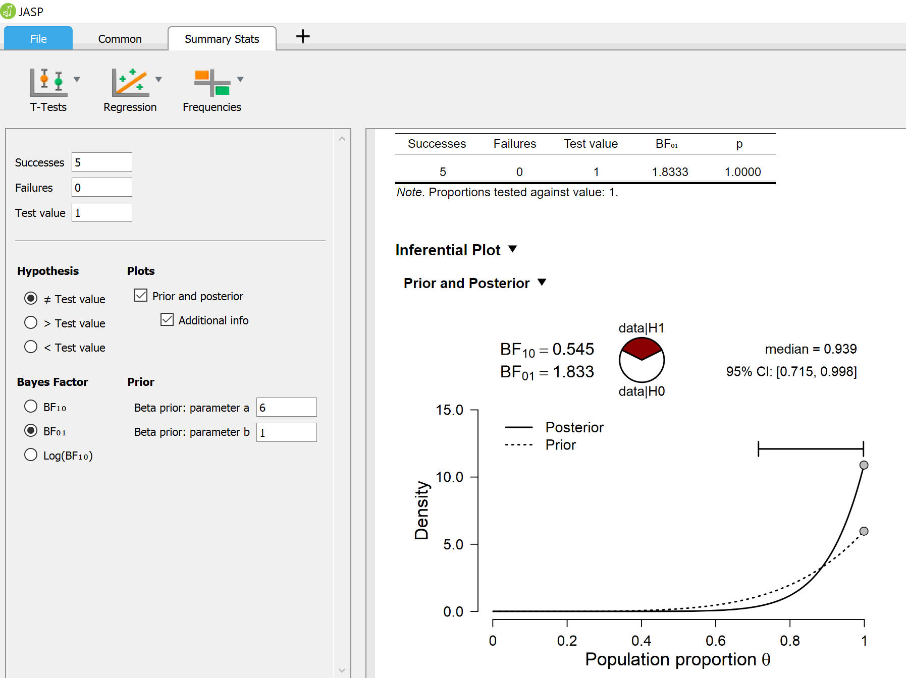
The result from Table 1 can be easily confirmed using the SumStat module in JASP (Ly et al., 2018 ). The screenshot below shows the results obtained when successes $= 5$ , failures $= 0$ , the test value is $\theta = 1$ , and the prior distribution is set to $a=6$ , $b=1$ . The Bayes factor in favor of the general law $\mathcal{H}_0$ equals $1.83$ .

Concluding Comments

As demonstrated above, posterior Bayes factors violate the fundamental inductive pattern. No matter how many apples one sees that grow from apple trees, no matter how many even integers greater than two are inspected that turn out to be the sum of two prime numbers, our confidence in these general laws would be bounded, and would forever remain caught in the evidential region that Jeffreys (1961, appendix B) called “not worth more than a bare mention”. This is preposterous.

The reason for such problematic behavior is the same as for LOO (Gronau et al., in press a, b): when two models are provided advance access to the data they are supposed to predict, this benefits the complex model much more than the simple model. If the data are consistent with the simple model, the complex model will abuse the advance access to the data to tune its parameters so that it effectively mimics the simple model; the comparison is then not between a complex model and a simple model, but between two simple and highly similar models — such a comparison cannot produce a diagnostic result.

In sum, we believe that models, hypotheses, and theories need to be assessed by the predictions that they make. Predictions, as the word suggests, need to come from the prior, not from the posterior. The famous Danish maxim tells us that “prediction is hard, particularly about the future”; the difficulty is real, but this does not license us to abandon the enterprise and start assessing our theories by postdiction instead.

Footnotes

¹ For a general beta $(a,b)$ prior, the limit of the posterior Bayes factor is $BF^{\star}_{01} = 2^b$ . See appendix for a derivation.

References

Aitkin, M. (1991). Posterior Bayes factors. Journal of the Royal Statistical Society. Series B (Methodological), 53, 111-142.

Gronau, Q. F., & Wagenmakers, E.-J. (in press a). Limitations of Bayesian leave-one-out cross-validation for model selection. Computational Brain & Behavior. Preprint.

Gronau, Q. F., & Wagenmakers, E.-J. (in press b). Rejoinder: More limitations of Bayesian leave-one-out cross-validation. Computational Brain & Behavior. Preprint.

Jeffreys, H. (1961). Theory of probability (3rd ed.). Oxford: Oxford University Press.

Ly, A., Raj, A., Etz, A., Marsman, M., Gronau, Q. F., & Wagenmakers, E.-J. (2018). Bayesian reanalyses from summary statistics: A guide for academic consumers. Advances in Methods and Practices in Psychological Science, 3, 367-374. Preprint; open access available through the journal website.

Polya, G. (1954). Mathematics and plausible reasoning: Vol. II. Patterns of plausible inference. Princeton, NJ: Princeton University Press.

Wendel, J. (1948). Note on the gamma function. The American Mathematical Monthly, 55, 563-564.

Appendix

Let $\theta$ denote the success probability of a binomial distribution and suppose that the $n$ observations are all successes. The posterior Bayes factor (Aitkin, 1991) for comparing the general law hypothesis $\mathcal{H}_0: \theta = 1$ to the alternative $\mathcal{H}_1: \theta \sim \text{beta}(a,b)$ is given by:

$\text{BF}^{\star}_{01} = \frac{\Gamma(a+n)}{\Gamma(a+n+b)} \thinspace \frac{\Gamma(a+2n+b)}{\Gamma(a+2n)}.$

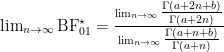
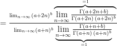
The limit of the posterior Bayes factor as $n$ goes to infinity is given by:

$\lim_{n \to \infty} \text{BF}^{\star}_{01} = \frac{\lim_{n \to \infty}\tfrac{\Gamma(a+2n+b)}{\Gamma(a+2n)}}{\lim_{n \to \infty}\tfrac{\Gamma(a+n+b)}{\Gamma(a+n)}}$

$= \frac{\lim_{n \to \infty}(a+2n)^b \, \overbrace{\lim_{n \to \infty}\tfrac{\Gamma(a+2n+b)}{\Gamma(a+2n) \, (a+2n)^b}}^{=1}}{\lim_{n \to \infty}(a+n)^b \, \underbrace{\lim_{n \to \infty}\tfrac{\Gamma(a+n+b)}{\Gamma(a+n) \, (a+n)^b}}_{=1}}$