In previous posts we provided detailed Bayesian reanalyses of two “p-just-below-.05” experiments (i.e., red, rank, and romance, and flag-priming). For both experiments, the evidence against the null hypothesis was relatively weak, and this supported the main claim from the paper “Redefine Statistical Significance” (and the 2016 claim by the American Statistical Association, and the claim made by statisticians throughout the last 60 years): one ought to approach p-values just below .05 with considerable caution. But how much caution? And what do we mean when we say that the evidence is “relatively weak”?
For concreteness, we will consider again the outcome from the one-sided Bayesian test of the flag-priming experiment (Figure 3 here). Recall that t(181) = 2.02, p = .045 (in words: “reject the null hypothesis” → “accept the claim in this manuscript” → “publish this article” → “from now on, let’s consider this finding Holy Writ”). The associated Bayes factor, however, was merely 2.062 (let’s just call that 2) in favor of H1. What this means is that the observed data are twice as likely under H1 than under H0. Harold Jeffreys called this level of evidence “not worth more than a bare mention”, but why? Isn’t this up for debate? Below are three scenarios that provide an intuition about the strength of the evidence that a Bayes factor provides. The scenarios are meant to be educational rather than realistic.
Scenario 1: Phil’s Sauna Dilemma
Phil visits a country that has 100 women-only saunas and 100 mixed saunas. The mixed saunas are frequented by 50% women and 50% men. After playing a few games of squash at the local club SquashVillage, Phil is eager to use their infrared sauna to ease the pains in his lower back. Unfortunately, Phil does not know whether the club’s sauna is women-only or mixed, and so he decides to play it safe and watch a few people enter and leave. The first person he sees existing the sauna is a woman. Under the mixed-sauna hypothesis, the probability of this outcome is .50, whereas under the women-only hypothesis the probability is 1. Consequently, Phil’s first observation yields a Bayes factor of 1/0.5 = 2 in favor of the “women-only” hypothesis.
Based on so little evidence, most of us would agree that it is premature for Phil to write an article in the premier journal Squash, Back Pain, & Sauna (SBPS) arguing that “the results from visually inspecting a single person exiting the SquashCity sauna supported my hypothesis and suggested that the sauna is women-only”. Clearly, Phil should observe more people exiting the sauna. The second person he sees is also a woman. This raises the Bayes factor to 2×2=4. A third person exists, again a woman; now the Bayes factor is 2x2x2=8. A fourth person exists and is also a woman: the Bayes factor is 16. A fifth woman appears, increasing the Bayes factor to 32.
Now ask yourself: how many consecutive women does Phil need to see exiting the sauna before he can feel sufficiently confident to write an influential SBPS article stating that “we reject the hypothesis that SquashVillage’s sauna is mixed”? In his 1997 book, Richard Royall formulated the sauna scenario more prosaically, in terms of an urn that is filled either with white marbles or with 50% white marbles and 50% black marbles. When we ask audiences how many consecutive white marbles need to be observed before they are comfortable writing a paper for the prestigious Urns, Marbles, and Dice (UMD) in which they reject the mixed-urn hypothesis, most people indicate either 4,5, or 6 consecutive marbles. Nobody has ever indicated 2 or lower.
[We would like to thank JP de Ruiter for suggesting the sauna interpretation of Royall’s urns.]Scenario 2: The Pepperoni-Mozzarella Pizza
We can also gauge the strength of the Bayes factor by calculating how much it changes our opinion given that we start from a position of indifference. Suppose that we deem H0 and H1 equally likely a priori (50%-50%). Observing a Bayes factor of 2 increases the plausibility of H1 to 2/3 ≈ 67% and leaves about 33% for H0. It does not seem prudent to reject H0 based on such evidence.
To make this more concrete we can visualize the updated plausibility estimates by means of a pizza plot, as we have discussed in our earlier blog posts. For the flag-priming example, we obtained the following result:
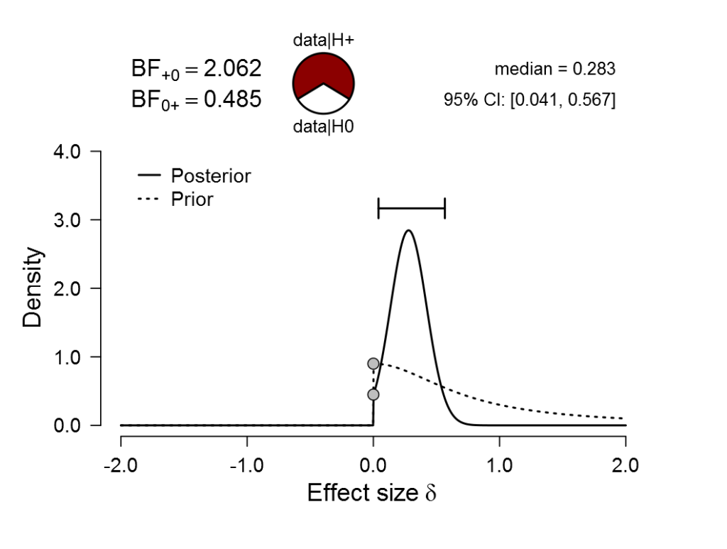
Figure 1. With a Bayes factor of 2 in favor of the alternative, and starting from a position of equipoise, the pepperoni (H1) covers two-thirds of the pizza, and the mozzarella (H0) covers the remaining one-third.
The pizza plot (commonly known as a probability wheel) on top of this figure indicates the 67% for H1 by the part covered in pepperoni, and the 33% for H0 by the part covered in mozzarella. To feel how much evidence this is, we may mentally execute the “Pizza-poke Assessment of the Weight of evidence” (PAW): if you pretend to poke your finger blindly in the pizza, how surprised are you if that finger returns covered in the non-dominant topping?
With equal prior odds, a Bayes factor of 8 results in a posterior probability of 8/9 ≈ 89% for pepperoni H1, leaving 11% for mozzarella H0. A Bayes factor of 16 results in 16/17 ≈ 94%, still leaving 6% for mozzarella H0.
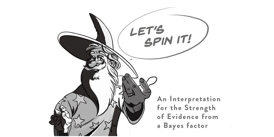
Scenario 3: A Wizard Spinning a Wheel
Created by our graphical artist Viktor Beekman, below is a cartoon of a wizard explaining the strength of evidence with a spinner. This is of course very similar to the PAW. The illustration uses a Bayes factor of 3 in favor of H1, which is near the maximum level of evidence that the Bayesian analyses (presented in “Redefine Statistical Significance“) provide for an experiment that yields a p-just-below-.05 result.
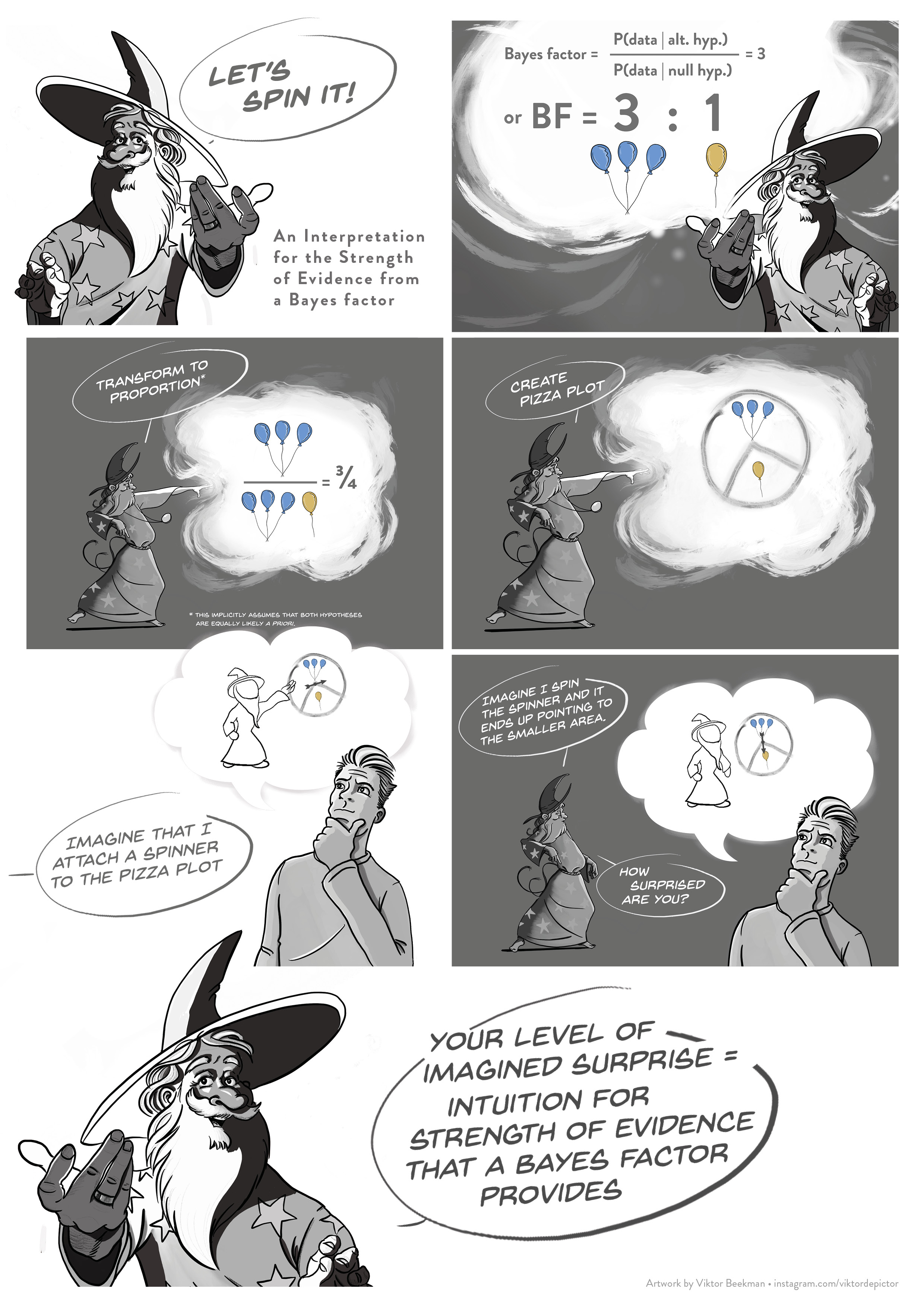
Figure 2. A wizard explains the strength of evidence (full picture here).
Take-home Messages
We have provided three scenarios –involving a sauna, a pizza, and a spinner– that provide an intuition for the strength of evidence that a Bayes factor provides. In all three scenarios, Bayes factors lower than 3 seem evidentially weak. It is apt to close with a quotation from Harold Jeffreys, one of the brightest scientific minds of the last century, who had spend much of his life working with Bayes factors. When confronted with a Bayes factor of 5.33 (hence: a PAW with 1/6.33 ≈ 16% mozzarella) Jeffreys remarked that these were “odds that would interest a gambler, but would be hardly worth more than a passing mention in a scientific paper” (Jeffreys, 1961, pp. 256-257). When such insights about evidence are translated to our current p-value threshold of .05, the result is sobering.
Like this post?
Subscribe to the JASP newsletter to receive regular updates about JASP including the latest Bayesian Spectacles blog posts! You can unsubscribe at any time.
References
Jeffreys, H. (1961). Theory of probability (3rd ed.). Oxford: Oxford University Press.
Royall, R. M. (1997). Statistical evidence: A likelihood paradigm. London: Chapman & Hall.
About The Authors

Eric-Jan Wagenmakers
Eric-Jan (EJ) Wagenmakers is professor at the Psychological Methods Group at the University of Amsterdam.

Quentin Gronau
Quentin is a PhD candidate at the Psychological Methods Group of the University of Amsterdam.