In the previous post we discussed the paper “Redefine Statistical Significance”. The key point of that paper was that p-values near .05 provide (at best) only weak evidence against the null hypothesis. This contradicts current practice, where p-values slightly lower than .05 bring forth an epistemic jamboree, one where researchers merrily draw bold conclusions such as “we reject the null hypothesis” (a champagne bottle pops in the background), “the effect is present” (four men in tuxedos jump in a pool), and “as predicted, the groups differ significantly” (speakers start blasting “We are the champions”). Unfortunately, these parties are premature – let’s say this again, because it is so important: p-values near .05 constitute only weak evidence against the null hypothesis. The following sentences from the paper bear repeating:
“A two-sided P-value of 0.05 corresponds to Bayes factors in favor of H1 that range from about 2.5 to 3.4 under reasonable assumptions about H1 (…) This is weak evidence from at least three perspectives. First, conventional Bayes factor categorizations (…) characterize this range as “weak” or “very weak.” Second, we suspect many scientists would guess that p ≈ 0.05 implies stronger support for H1 than a Bayes factor of 2.5 to 3.4. Third, using (…) a prior odds of 1:10, a P-value of 0.05 corresponds to at least 3:1 odds (…) in favor of the null hypothesis!”
In the ensuing online discussions, many commentators did not properly appreciate the severity of the situation. Perhaps this is because the arguments from the paper were too abstract, or because the commentators had not managed to escape from the mental gulag that is commonly referred to as Neyman-Pearson hypothesis testing. The purpose of this post is to discuss a concrete example of a pool party based on p-near-.05, and show why the party is premature.
Red, Rank, and Romance in Women Viewing Men
In a 2010 article published in the prestigious Journal of Experimental Psychology: General (JEP:Gen), a group of seven researchers conducted a series of experiments that
“demonstrate that women perceive men to be more attractive and sexually desirable when seen on a red background and in red clothing, and we additionally show that status perceptions are responsible for this red effect.” (Elliot et al., 2010, p. 399).
DISCLAIMER: We use this work to demonstrate a general statistical regularity, namely that p-values near .05 provide only weak evidence; we do not wish to question the veracity of the entire body of work (for a discussion see Francis, 2013; Elliot & Maier, 2013) nor the author’s moral compass. Indeed, any article with a key p-value near .05 would have served our purpose just as well. We chose this article because the hypothesis speaks to the imagination and the experimental design is easy to explain.
Here we focus on the first experiment, in which two groups of female undergraduates were asked to rate the attractiveness of a single male from a black-and-white photo. Ten women saw the photo on a red background, and eleven women saw the photo on a white background. The authors analyzed the data and interpreted the results as follows:
“An independent-samples t test examining the influence of color condition on perceived attractiveness revealed a significant color effect, t(20) = 2.18, p<.05, d=0.95 (…) Participants in the red condition, compared with those in the white condition, rated the target man as more attractive (M = 6.79, SD = 1.00, and M = 5.67, SD = 1.34, respectively). None of the participants correctly guessed the purpose of the experiment. Thus, the results from this experiment supported our hypothesis and suggested that color influences participants’ ratings without their awareness.”
But how strong is this suggestion? Let’s turn to a Bayesian analysis to find out (TL;DR: the suggestion is not compelling, irrespective of the details of the analysis).
A Bayesian Reanalysis Using JASP
For our Bayesian reanalysis we use the Summary Stats module in the free software package JASP (jasp-stats.org; see also Ly et al., 2017). Undeterred by why the independent-samples t-test has 20 degrees of freedom, we proceed to enter “2.18” in the box for the t-value, “10” in the box for “Group 1 size” and “11” in the box for “Group 2 size”. A screenshot of the JASP input panel is here. The resulting table output shows that the p-value equals .042.
To obtain a more detailed view we request a “Prior and posterior” plot with “Additional info”. The result, obtained with two mouse clicks:
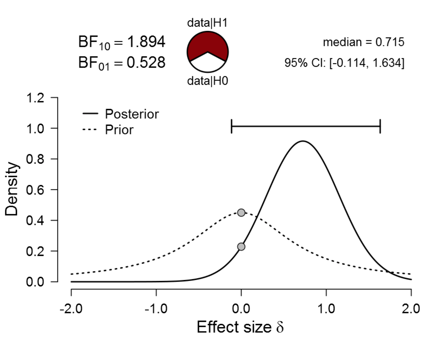
Figure 1. Bayesian reanalysis of data that give t(20) = 2.18, p = .042. The prior under H1 is a default Cauchy distribution with location 0 and scale 0.707. The evidence for H1 is weak. Figure from JASP.
The dotted line is the default “Cauchy distribution” prior distribution for effect size under H1: the most likely effect sizes are near zero, but large effect sizes are also possible (for details see Ly et al., 2016). The solid line is the posterior distribution for effect size under H1: the posterior median is 0.715, and 95% of the posterior mass falls between -0.114 and 1.634. Under the assumption that H1 is the true model, we know that the effect size (1) has not been estimated with much precision; (2) is probably positive rather than negative. Crucially, however, we do not want to assume that H1 is true from the outset, as this would be begging the question.
The p-value hypothesis test evaluates the skeptic’s point null hypothesis H0: effect size delta = 0, and we will do the same, but now from within a Bayesian framework. This means that we contrast the predictive performance of two competing hypotheses: the point null hypothesis H0 (i.e., a spike at delta = 0) and the alternative hypothesis H1 (i.e., the dotted default Cauchy distribution prior shown in the above figure). The result is a Bayes factor that equals 1.89. In other words, the observed data are about twice as likely to occur under the default alternative hypothesis than under the null hypothesis.
The strength of this evidence is visualized by means of the pizza plot on top of the figure. In a starting position of equipoise, half of the pizza is covered with pepperoni (red; H1), and the other half with mozzarella (white; H0). After seeing the data, the pepperoni part has increased somewhat, but there remains a sizable mozzarella part. In other words, if you blindly poke your finger in the pizza, you would not be terribly surprised if returned covered in mozzarella. Let’s call this the “Pizza-poke Assessment of the Weight of evidence” (PAW).
This initial reanalysis corroborates the main claim from the Redefine Statistical Significance paper –and the 2016 statement by the American Statistical Association– that p-values near .05 are weak evidence. However, we used a default prior to quantify the expectations for effect size under H1. We will now follow Bem’s adage and “examine the data from every angle” and apply a broad range of priors to gauge the extent to which this changes the results. WARNING: A full realization of the weakness of the evidence can be shocking and change the way you view p-values. Those who cannot stomach the evidential carnage are advised to skip ahead to the take-home messages.
But What About the Width of the Prior Distribution for Effect Size under H1?
In the JASP Summary Stats module, we select “Bayes factor robustness check” with “Additional info” and, with two mouse clicks, obtain the following outcome:
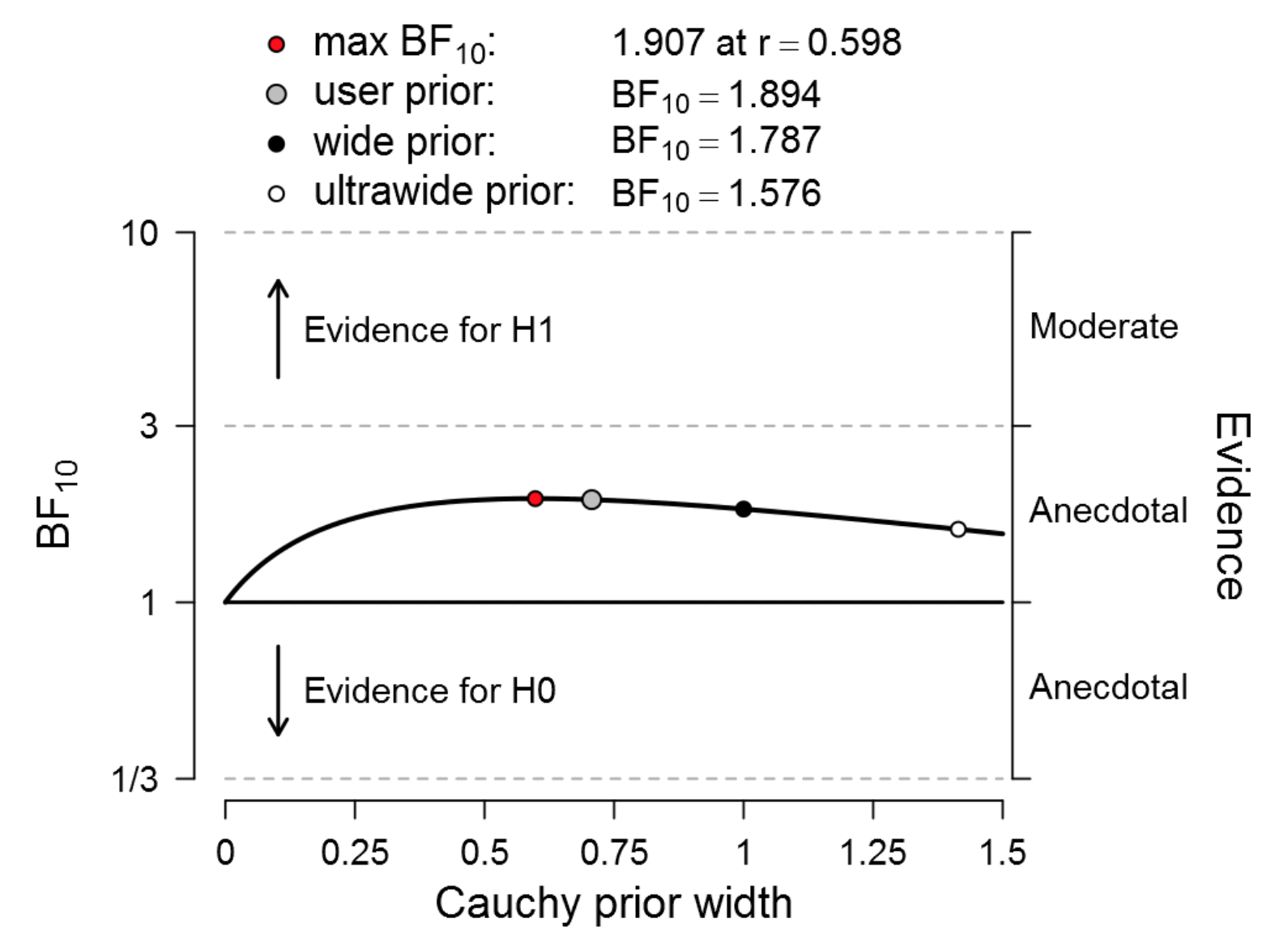
Figure 2. Bayesian robustness analysis of data that give t(20) = 2.18, p = .042. The prior under H1 is a default Cauchy distribution with location 0 and the scale varies as indicated on the x-axis. The evidence for H1 is weak regardless of the prior width. Figure from JASP.
This ought to be deeply disturbing. Even when we cheat to cherry-pick the prior width that governs the expectations for effect size under H1, the Bayes factor does not exceed 2. In the language of Harold Jeffreys, this evidence is “not worth more than a bare mention”.
But What Happens When We Conduct a One-Sided Test?
This is a valid point. The authors’ hypothesis predicts that the color red increases attractiveness; it does not predict that the color red decreases attractiveness. In lieu of the two-sided nature of the authors’ own analysis, we conduct a one-sided test by selecting “Group 1 > Group 2” in the JASP Summary Stats module. The result:
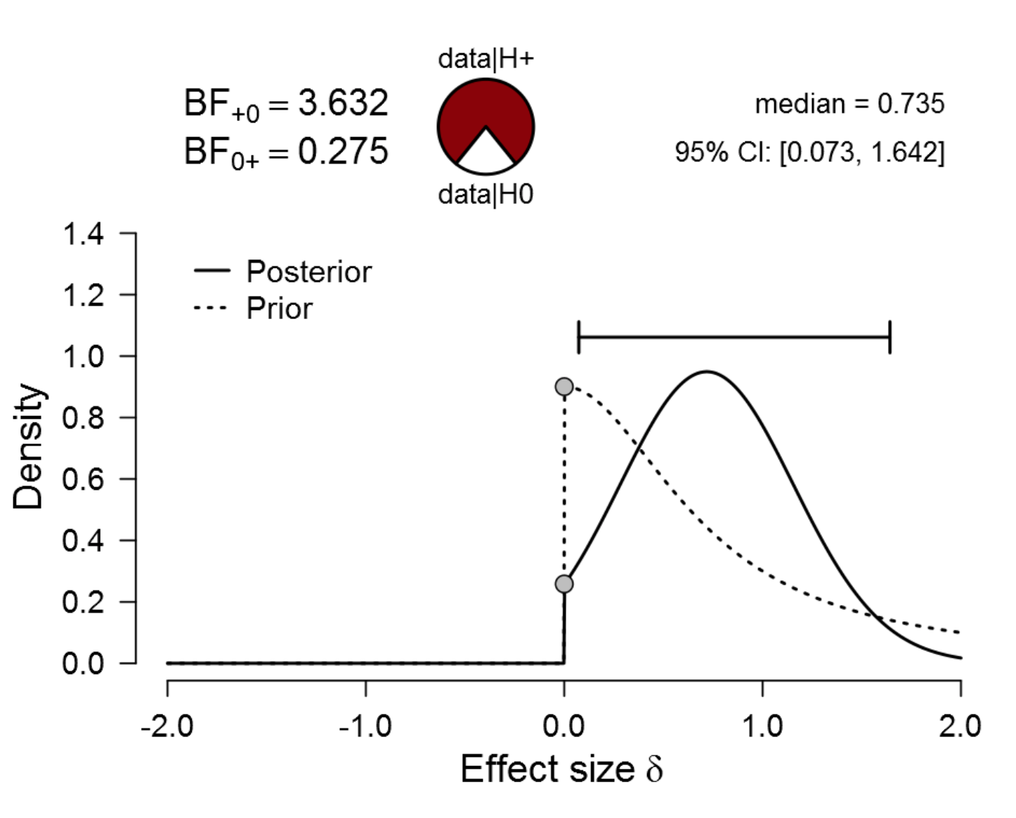
Figure 3. Bayesian reanalysis of data that give t(20) = 2.18, p = .042. The prior under H1 is a one-sided default Cauchy distribution with location 0 and scale 0.707. The evidence for H1 is still not compelling. Figure from JASP.
The one-sided analysis has increased the evidence in favor of the alternative hypothesis almost by a factor of two, and the Bayes factor is now 3.632. The weight of this evidence is again indicated by the pizza plot. Mentally conduct your own PAW and it is obvious that any claims need to be accompanied by modesty and caution.
Hey, Why Aren’t You Showing the Robustness Analysis for the One-Sided Test?
Alright, you asked for it:
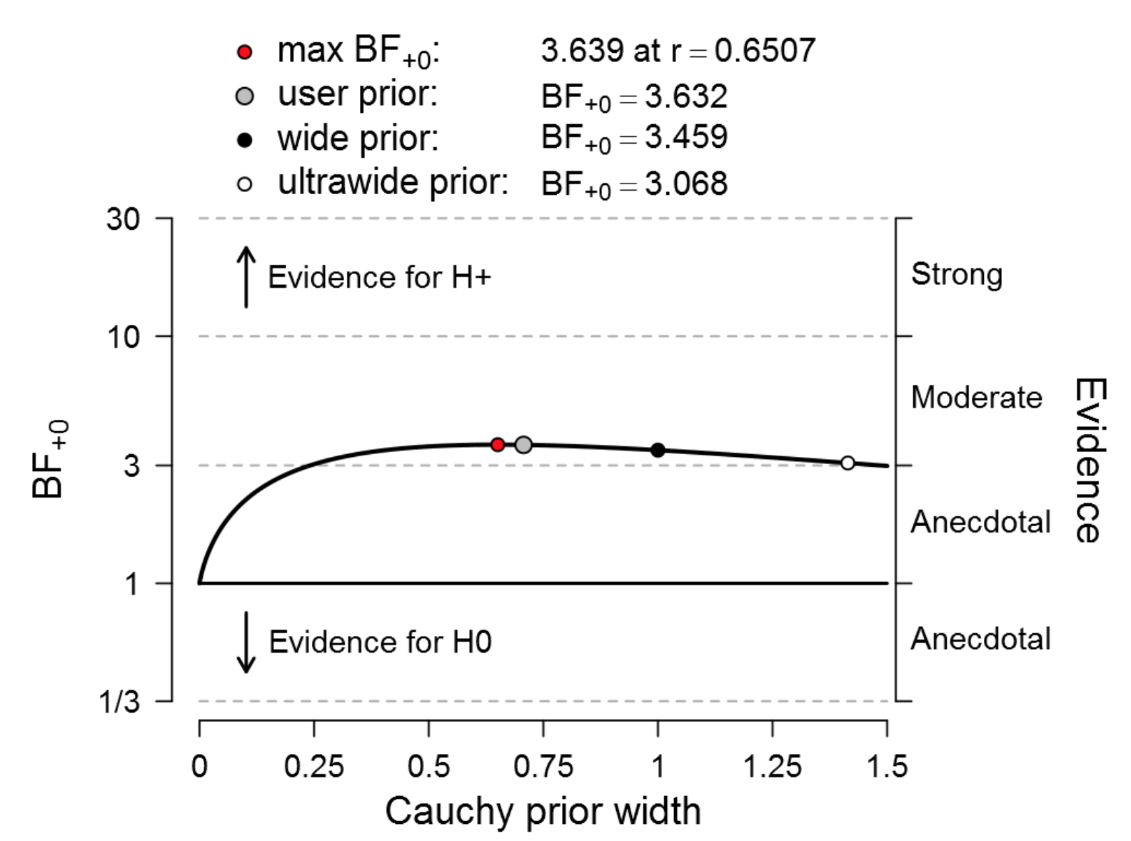
Figure 4. Bayesian robustness analysis of data that give t(20) = 2.18, p = .042. The prior under H1 is a one-sided default Cauchy distribution with location 0 and the scale varies as indicated on the x-axis. The evidence for H1 is not compelling regardless of the prior width. Figure from JASP.
When we cherry-pick the prior width to provide the strongest evidence against H0, that evidence is only 3.639, almost identical to the evidence obtained from the default width of 0.707.
What About Priors That Are Not Centered on Zero?
Virtually all existing Bayesian hypothesis testing and model selection procedures use prior distributions that are centered around the value under test. JASP is no exception, and the current JASP Summary Stats module does not provide the flexibility to use priors centered away from zero. However, the next version of JASP overcomes this limitation and offers a range of prior distributions that can be centered away from zero (see Gronau et al., 2017). The next blog post (part III – we expect to continue the series for a while) will investigate whether the evidence is more compelling when these “informed priors” are used.
Take-Home Messages
Here we provided just one concrete example showcasing how little evidence is provided by a p=.042 result. In future blog posts, we will provide many more examples, featuring work on important topics published in the highest impact journals. Hopefully the example discussed above has already provided a better idea of why the .05 threshold is dangerously lenient, easily allowing spurious findings to infest the literature. We end with a few conclusions.
- The Summary Stats module in JASP is a promising new tool to reanalyze findings from the literature when the raw data are not available. From just a few mouse clicks and keystrokes, JASP produces a comprehensive Bayesian evaluation that goes considerably beyond summaries such as “t(20) = 2.18, p = .042”. If you want to learn more about Bayesian analyses in JASP you can still register for our Awesome August workshop, co-taught with Richard Morey.
- In our example the Bayes factors still supported the alternative hypothesis. It is just that the degree of this support is disappointing. So although p-values near .05 may not be worthy of a jamboree, they should also not lead researchers to prematurely bury a hypothesis either. It is unfortunate that the frequentist
gulagframework forces researchers to adopt a mindset in which an experiment results either in a jamboree or in a funeral. Such all-or-none decision making does not do justice to the continuous nature of the evidence. Many p-near-.05 results should inspire neither jamboree nor funeral; instead, they should be taken as preliminary encouragement to explore the matter more deeply. - The current .05 threshold is a fly-trap for researchers. The criterion itself (“1-in-20”) instills a false sense of security, and leads researchers to make bold claims that misrepresent the evidence, thereby fooling themselves, their readership, and society at large. This needs to stop. Strong claims require strong evidence, and p-values near .05 simply don’t have what it takes.
In sum, the field’s infatuation with the lenient .05 threshold is highly problematic. We have been caught in a bad romance, and it is time to take back control.
Like this post?
Subscribe to the JASP newsletter to receive regular updates about JASP including the latest Bayesian Spectacles blog posts! You can unsubscribe at any time.
References
Elliot, A. J., Kayser, D. N., Greitemeyer, T., Lichtenfeld, S., Gramzow, R. H., Maier, M. A., Liu, H. (2010). Red, rank, and romance in women viewing men. Journal of Experimental Psychology: General, 139, 399-417.
Elliot, A. J., & Maier, M. A. (2013). The red-attractiveness effect, applying the Ioannidis and Trikalinos (2007b) test, and the broader scientific context: A reply to Francis (2013). Journal of Experimental Psychology: General, 142, 297-300.
Francis, G. (2013). Publication bias in “Red, Rank, and Romance in Women Viewing Men,” by Elliot et al. (2010). Journal of Experimental Psychology: General, 142, 292-296.
Gronau, Q. F., Ly, A., & Wagenmakers, E.-J. (2017). Informed Bayesian t-tests. Manuscripts submitted for publication. Available at https://arxiv.org/abs/1704.02479.
Ly, A., Verhagen, A. J., & Wagenmakers, E.-J. (2016). Harold Jeffreys’s default Bayes factor hypothesis Tests: Explanation, extension, and application in psychology. Journal of Mathematical Psychology, 72, 19-32.
Ly, A., Raj, A., Marsman, M., Etz, A., & Wagenmakers, E.-J. (2017). Bayesian reanalyses from summary statistics: A guide for academic consumers. Manuscript submitted for publication. Available at https://osf.io/7t2jd/.
Wagenmakers, E.-J., Verhagen, A. J., Ly, A., Matzke, D., Steingroever, H., Rouder, J. N., & Morey, R. D. (2017). The need for Bayesian hypothesis testing in psychological science. In Lilienfeld, S. O., & Waldman, I. (Eds.), Psychological Science Under Scrutiny: Recent Challenges and Proposed Solutions, pp. 123-138. John Wiley and Sons.
About The Authors

Eric-Jan Wagenmakers
Eric-Jan (EJ) Wagenmakers is professor at the Psychological Methods Group at the University of Amsterdam.

Quentin Gronau
Quentin is a PhD candidate at the Psychological Methods Group of the University of Amsterdam.