In the two previous posts on the paper “Redefine Statistical Significance”, we reanalyzed Experiment 1 from “Red, Rank, and Romance in Women Viewing Men” (Elliot et al., 2010). Female undergrads rated the attractiveness of a single male from a black-and-white photo. Ten women saw the photo on a red background, and eleven saw the photo on a white background. The results showed that “Participants in the red condition, compared with those in the white condition, rated the target man as more attractive”; in stats speak, the authors found “a significant color effect, t(20) = 2.18, p<.05, d=0.95”. However, our Bayesian reanalysis with the JASP Summary Stats module (jasp-stats.org ) revealed that this result provides only modest evidence against the null hypothesis, even when the prior distributions under H1 are cherry-picked to present the most compelling case.
At this point the critical reader may wonder whether our demonstration works because Elliot et al. tested only 21 participants. Perhaps p-values near .05 yield convincing evidence when sample size is larger, such that effect size can be estimated accurately. We will evaluate this claim by examining another concrete example: flag priming.
Flag priming
In Experiment 1 of their article “A Single Exposure to the American Flag Shifts Support Toward Republicanism up to 8 Months Later”, Carter et al. (2011)
“(…) tested whether a single exposure to the American flag would lead participants to shift their attitudes, beliefs, and behavior in the politically conservative direction. We conducted a multisession study during the 2008 U.S. presidential election.”
The study featured various outcome measures and analyses, but for the purposes of this statistical demonstration we focus on the following result:
“As predicted, participants in the flag-prime condition (M = 0.072, SD = 0.47) reported a greater intention to vote for McCain than did participants in the control condition (M = -0.070, SD = 0.48), t(181) = 2.02, p = .04, d = 0.298.”
We assume that the total sample size was 183, and that there were 92 people in the flag-prime condition and 91 in the control condition. How strong is the evidence that corresponds to this “p=.04” result? Let’s conduct a Bayesian reanalysis in JASP and find out.
DISCLAIMER: We use this work to demonstrate a general statistical regularity, namely that p-values near .05 provide only weak evidence; we do not wish to question the veracity of the entire body of work (for a “many labs” replication attempt see Klein et al., 2014), and we do not question the moral compass of the authors. Indeed, any article with a key p-value near .05 would have served our purpose just as well. We choose this article because the experiment speaks to the imagination and is easy to explain.
Bayesian Reanalysis of the Flag Priming Experiment
Using the Summary Stats module in JASP, we select “Bayesian Independent Samples T-Test” and then enter “2.02” in the box for the t-value, “92” in the box for “Group 1 size” and “91” in the box for “Group 2 size”. The resulting table output shows that the p-value equals .045, similar in value to the p-value of .042 from the earlier Red, Rank, and Romance example. A screenshot of the JASP input panel is here.
To obtain a more detailed view we request a “Prior and posterior” plot with “Additional info”. The result, obtained with two mouse clicks:
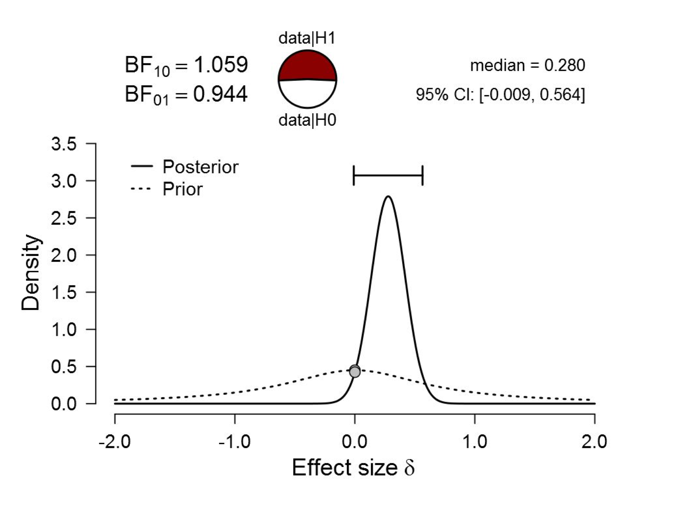
Figure 1. Bayesian reanalysis of data that give t(181) = 2.02, p = .045. The prior under H1 is a default Cauchy with location 0 and scale 0.707. There is virtually no evidence for H1. Figure from JASP.
The default Bayes factor BF10 is almost exactly 1, meaning that the data are almost perfectly ambivalent. In other words, the null hypothesis and the default alternative hypothesis predict the observed data equally well.
This example suggests that for p-values near .05, large sample sizes do not alleviate the evidential crisis. Instead, they deepen this crisis. With p-values near .05, large samples indicate small effect sizes, and this benefits the null hypothesis.
The weakness of the evidence is on full display when we select “Bayes factor robustness check” with “Additional info”. With two mouse clicks, we obtain the following outcome:
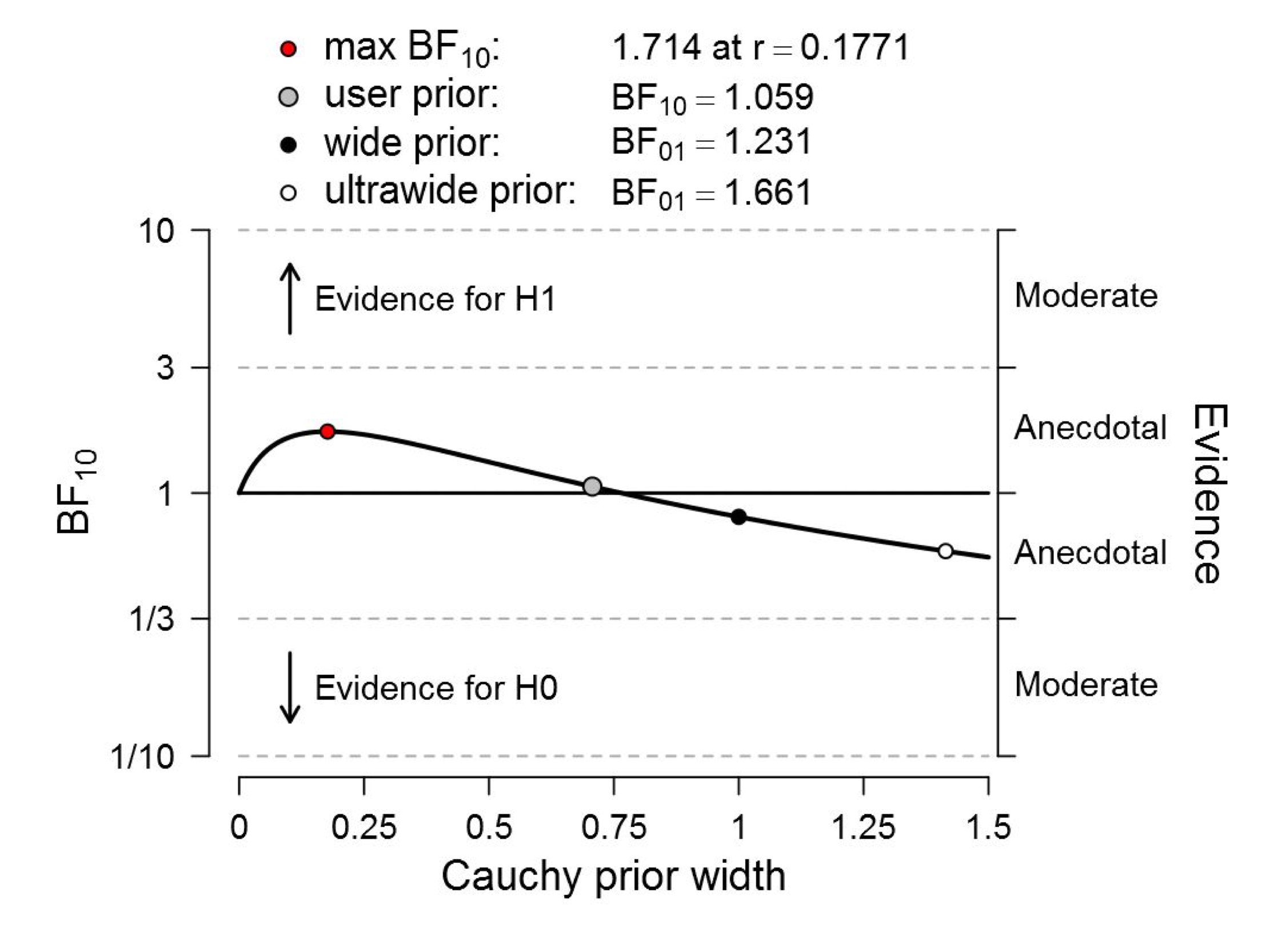
Figure 2. Bayesian robustness analysis of data that give t(181) = 2.02, p = .045. The prior under H1 is a default Cauchy with location 0 and the scale varies as indicated on the x-axis. There is hardly any evidence for H1, irrespective of the prior width. Figure from JASP.
This result is even more disturbing than it was for Red, Rank, and Romance. Even when we cheat to cherry-pick the prior width that governs the expectations for effect size under H1, the Bayes factor does not exceed 1.8.
To get a more complete impression of how weak the evidence really is, we will now proceed to use a series of alternative prior distributions under H1.
First we can apply a one-sided test, and truncate the prior distribution under H1 so that it only predicts positive effect sizes. This is accomplished in JASP with a single mouse click, and this is the result:
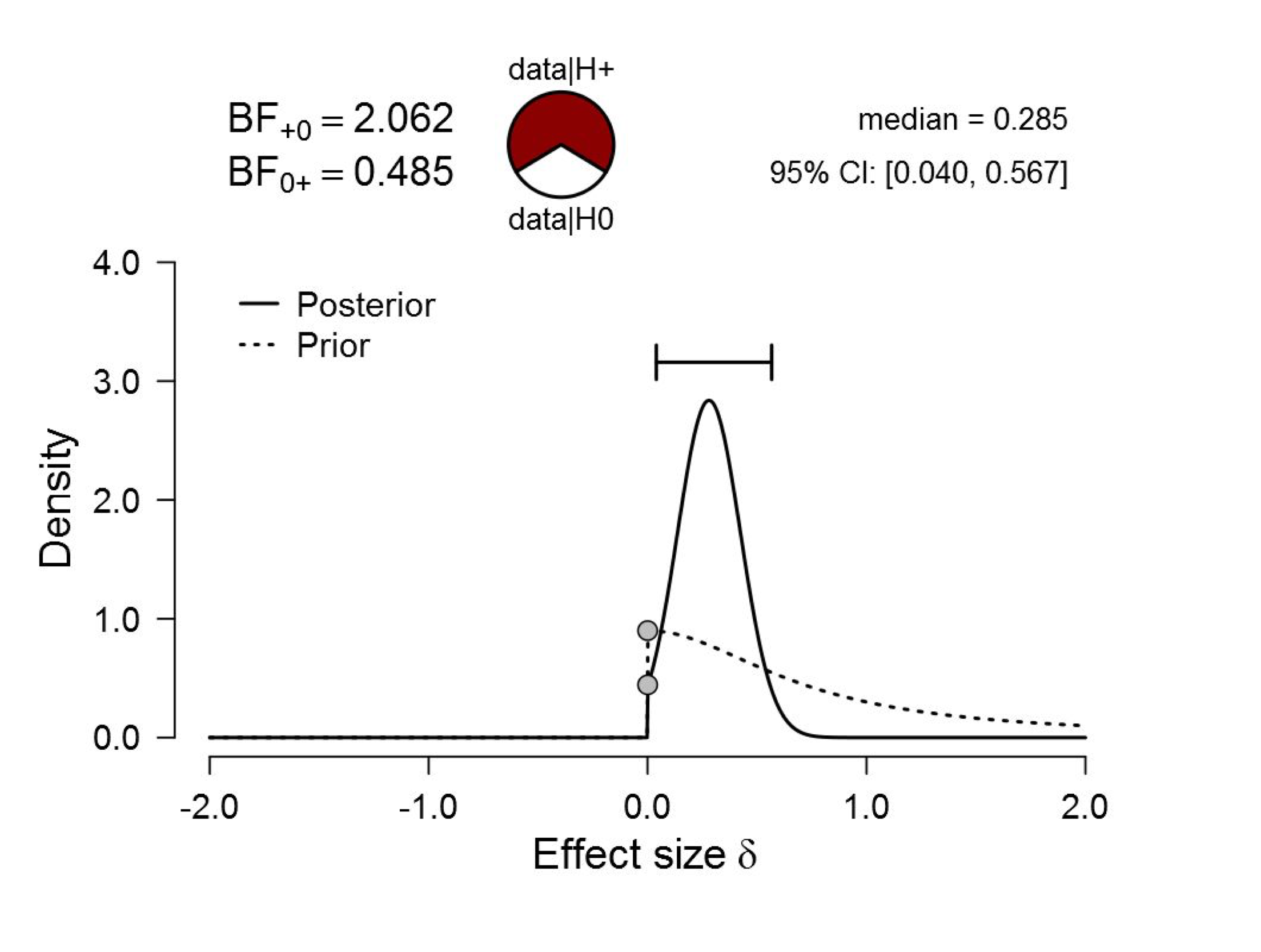
Figure 3. Bayesian reanalysis of data that give t(181) = 2.02, p = .045. The prior under H1 is a one-sided default Cauchy with location 0 and scale 0.707. The evidence for H1 is still weak. Figure from JASP.
Imposing the restriction to positive effect sizes increases the average predictive performance of H1, but the Bayes factor is still only 2. In the next blog post we will examine in detail how weak such a level of evidence really is, but here we will just mention that if the prior plausibility for H1 vs. H0 was 50% a priori, a Bayes factor of 2 has increased it to a mere 66.6%. That leaves a full 33.3% for H0.
For the one-sided analysis we can again conduct a robustness analysis:
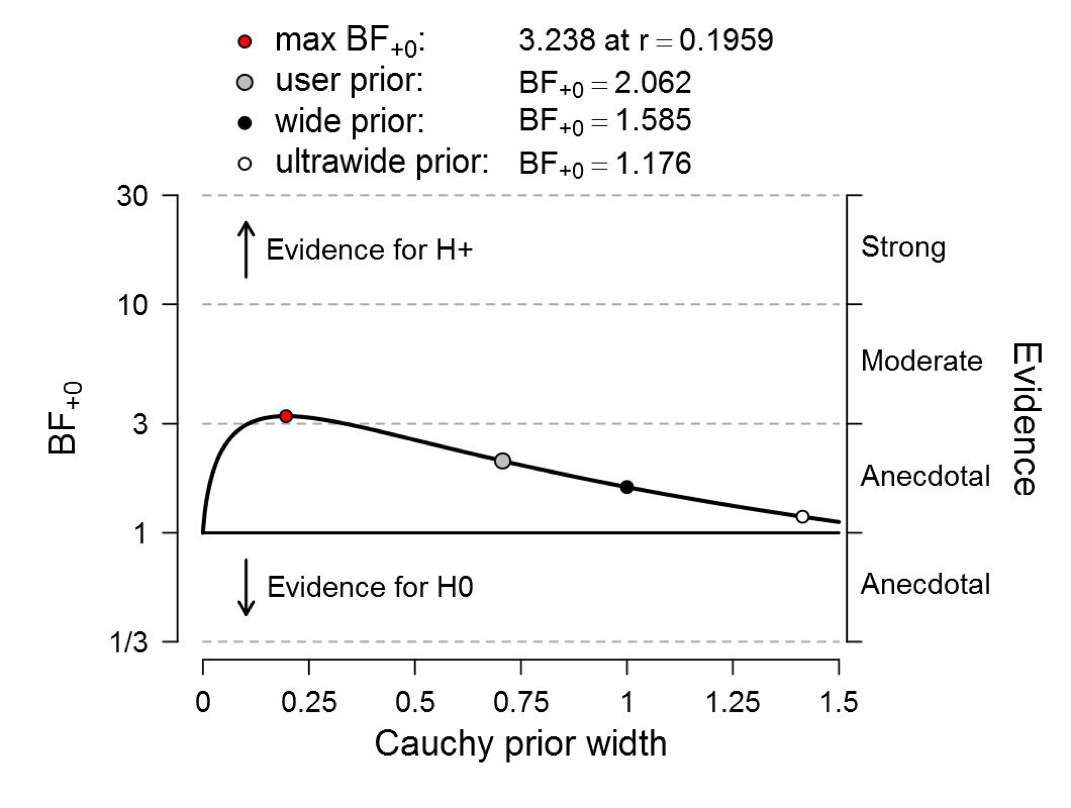
Figure 4. Bayesian robustness analysis of data that give t(181) = 2.02, p = .045. The prior under H1 is a one-sided default Cauchy with location 0 and the scale varies as indicated on the x-axis. The evidence for H1 remains unconvincing, irrespective of the prior width. Figure from JASP.
Even if we cherry-pick the scale of the one-sided prior distribution to be about 0.20, the maximum Bayes factor is only about 3.2. This means that this evidence increases the prior plausibility from 50% to 76%; a noticeable increase but one that still leaves a whopping 24% for the null hypothesis. To “reject the null hypothesis” based on such flimsy evidence is scientifically irresponsible.
Informed Priors and Oracle Priors
We first turn to an informed prior. We apply the Oosterwijk prior that we feel is particularly suited for general small-to-medium size effects. Note that this functionality is available from JASP 0.8.2 onward. The Oosterwijk prior is quantitatively in line with the observed effect size in the flag priming study, so it may be expected that the evidence will now be compelling. A few keystrokes and mouse clicks yield the result:
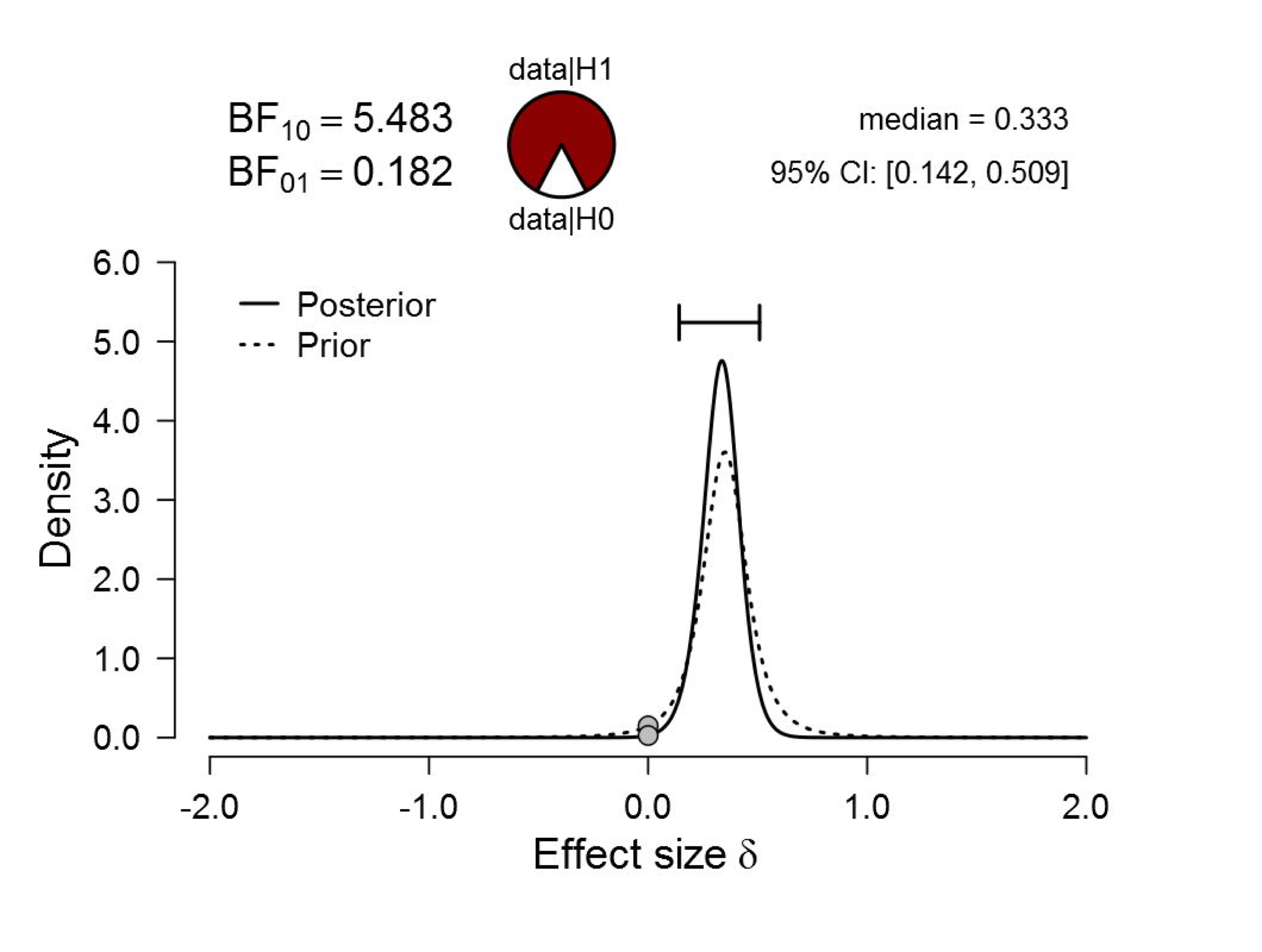
Figure 5. Bayesian reanalysis of data that give t(181) = 2.02, p = .045. The prior under H1 is the Oosterwijk t-distribution with location 0.35, scale 0.102, and 3 degrees of freedom. The evidence for H1 is much less compelling than the p-value suggests. Figure from JASP.
Under the Oosterwijk prior, the Bayes factor is now about 5.5. Note that the prior distribution is relatively strong, and the data have therefore caused only a modest update. Nevertheless, the alternative hypothesis has predicted the observed data about 5.5 times better than the null hypothesis. Before sending out the party invitations it is prudent to assess how much evidence this really is. With a prior plausibility for H1 vs. H0 of 50%, this Bayes factor will increase that plausibility to 84.6%. This leaves 15.4% for the null hypothesis. Should this be the level of evidence that our field aspires to when we “reject the null hypothesis”? We seriously doubt that researchers would be on board with this. The p=.045 (“less than 1-in-20”) result certainly seems to suggest a much stronger level of evidence, and this fools researchers into believing the evidence from the literature is more compelling than it really is.
Finally we apply an oracle prior and center the prior distribution on the observed effect size, d = 0.298. In the absence of crystal balls and ESP, this is preposterous. We first use a normal prior distribution centered at 0.298 and with standard deviation 0.1, such that 68% of the prior mass falls between 0.198 and 0.398. The result:

Figure 6. Bayesian reanalysis of data that give t(181) = 2.02, p = .045. The prior under H1 is a Normal distribution with mean 0.298 (i.e., the observed effect size) and standard deviation 0.1. The evidence for H1 is much less compelling than the p-value suggests, and the prior distribution is implausible. Figure from JASP.
The result is numerically close to that of the Oosterwijk prior. These data would update a 50% plausibility for H1 vs. H0 to 86%, leaving 14% for the null hypothesis.
An absolute bound can be obtained by assigning all prior mass to the observed effect size, that is, a normal distribution with mean d=.298 and standard deviation 0. This yields a Bayes factor of 7.56. This absolute maximum updates a 50% plausibility for H1 vs. H0 to 88%, leaving 12% for the null hypothesis. This is still not as compelling as p=.042 suggests. Moreover, the prior is beyond preposterous (is there even a word for that?). Using the beyond-preposterous prior but conducting a two-sided test (i.e., with half of the prior mass on d=-.298 and half on d=.298) instead of a one-sided test already reduces the Bayes factor to about 3.5. The party invitations will have to be put on hold.
Take-home Message
With p-values near .05, large sample sizes correspond to evidence that is even less compelling than was obtained for small sample sizes. Even the strongest prejudice against the null hypothesis cannot warrant the kinds of blanket statements that accompany p-values near .05.
The flag priming example underscores the recommendation from the paper “Redefine Statistical Significance”: p-values near .05 need to be treated with caution and modesty.
Generally, we believe that we can do better than a p-value, regardless of what threshold we choose or what label we attach. With a few mouse clicks in JASP, one can report the evidence, the posterior distribution, the prior distribution, and assess the robustness of the results. This comprehensive analysis provides a statistical overview that is more informative and useful than the one that is now standard.
In our next blog post, we will discuss how mixed-sex saunas can provide an intuition for the strength of evidence that a Bayes factor provides. Stay tuned.
Like this post?
Subscribe to the JASP newsletter to receive regular updates about JASP including the latest Bayesian Spectacles blog posts! You can unsubscribe at any time.
References
Carter, T. J., Ferguson, M. J., Hassin, R. R. (2011). A single exposure to the American flag shifts support toward Republicanism up to 8 months later. Psychological Science, 22, 1011-1018.
Elliot, A. J., Kayser, D. N., Greitemeyer, T., Lichtenfeld, S., Gramzow, R. H., Maier, M. A., Liu, H. (2010). Red, rank, and romance in women viewing men. Journal of Experimental Psychology: General, 139, 399-417.
Gronau, Q. F., Ly, A., & Wagenmakers, E.-J. (2017). Informed Bayesian t-tests. Manuscripts submitted for publication. Available at https://arxiv.org/abs/1704.02479.
Klein, R. A., et al. (2014). Investigating variation in replicability: A “many labs” replication project. Social Psychology, 45, 142-152.
Ly, A., Raj, A., Marsman, M., Etz, A., & Wagenmakers, E.-J. (2017). Bayesian reanalyses from summary statistics: A guide for academic consumers. Manuscript submitted for publication. Available at https://osf.io/7t2jd/.
About The Authors

Eric-Jan Wagenmakers
Eric-Jan (EJ) Wagenmakers is professor at the Psychological Methods Group at the University of Amsterdam.

Quentin Gronau
Quentin is a PhD candidate at the Psychological Methods Group of the University of Amsterdam.