Has the common criterion for statistical significance –“1-in-20”– tempted researchers into making strong claims from weak evidence? Should p-values near .05 be considered only suggestive? Are researchers caught in a bad romance? Last year, the American Statistical Association stated that “a p-value near 0.05 taken by itself offers only weak evidence against the null hypothesis” (Wasserstein and Lazar, 2016, p. 132), suggesting that the ASA believes the answers to be affirmative. The ramifications of the field’s infatuation with the .05 threshold are profound.
Revisiting Red, Rank, and Romance in Women Viewing Men
In the previous post we illustrated the ASA statement (and the more elaborate statement from the recent paper “Redefine statistical significance” with a concrete example. Specifically, we considered Experiment 1 from “Red, Rank, and Romance in Women Viewing Men” by Elliot et al. (2010). In this experiment, 21 female undergrads rated the attractiveness of a single male from a black-and-white photo. Ten women saw the photo on a red background, and eleven women saw the photo on a white background. The authors analyzed the data and interpreted the results as follows:
“An independent-samples t test examining the influence of color condition on perceived attractiveness revealed a significant color effect, t(20) = 2.18, p<.05, d=0.95 (…) Participants in the red condition, compared with those in the white condition, rated the target man as more attractive (…)”
In the previous post, we used the Summary Stats module in the free software package JASP (jasp-stats.org; see also Ly et al., 2017) and subjected these results to a Bayesian reanalysis. Part of this reanalysis contrasted predictive performance of the null hypothesis (effect size = zero) against that of an alternative hypothesis. Comparing the predictive adequacy of these two hypotheses yields the evidence, that is, the degree to which the data should change our mind. The evidence is also known as the Bayes factor.
The main challenge of the Bayes factor reanalysis is to specify the “prior distribution”, in this case the expectations for effect size under H1. The near-universal approach in Bayesian statistics is to center that prior on the value at test. As shown in the previous post, this default analysis did not produce compelling evidence against the null hypothesis, irrespective of the width of the prior distribution. Conducting a one-sided test increased the evidence, but it still does not warrant the kind of enthusiasm that usually accompanies a p=.042 result.
We now examine what happens when we allow the prior distributions to be centered on values that differ from zero (see Gronau et al., 2017). We will again use the Summary Stats module in JASP, but note that the “informed prior” analyses are available only in the upcoming version, that is, JASP 0.8.2.
The Oosterwijk Prior
The first informed prior we examine is the one we have elicited from Dr. Suzanne Oosterwijk, a social psychologist at the University of Amsterdam. This “Oosterwijk prior” captures the expert opinion for a specific effect, but we believe it is a plausible prior to quantify expectations about a small-to-medium size effect in experimental psychology more generally. The Oosterwijk prior is a t-distribution with location 0.350, scale 0.102, and 3 degrees of freedom. A screenshot of the JASP 0.8.2 input panel for this informed prior distributions is here. Applying the Oosterwijk prior to the analysis of the Elliot et al. “red and romance” data yields the following result:
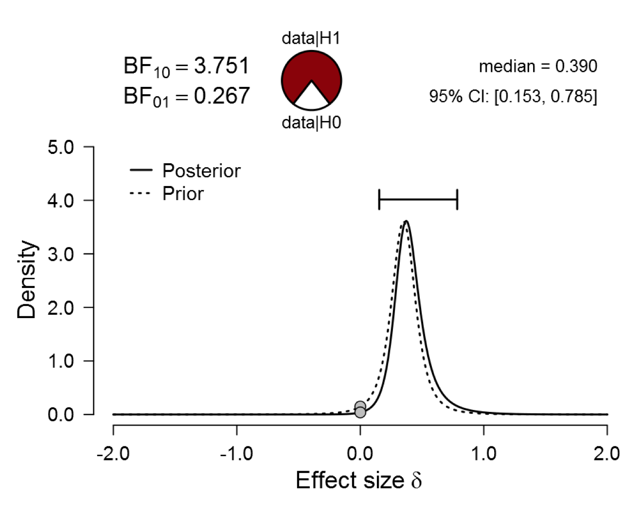
Figure 1. Bayesian reanalysis of data that give t(20) = 2.18, p = .042. The prior under H1 is the Oosterwijk t-distribution with location 0.35, scale 0.102, and 3 degrees of freedom. The evidence for H1 remains unconvincing. Figure from JASP.
As the figure shows, the Oosterwijk prior (dotted line) assigns most mass to effect sizes from 0.1 to about 0.6. Because this prior is highly informative, the data cause only a modest update in beliefs; the end result is a posterior distribution (solid line) that is relatively similar to the prior distribution.
REMARK 1. Note the posterior distribution is relatively peaked and located away from zero. Nevertheless, the data have caused only a small update in beliefs, suggesting that the evidence coming from the data is modest. Importantly, if exactly the same posterior distribution had been obtained from a prior that was much more spread out, then the evidence would have been compelling. The upshot is that the assessment of evidence cannot be based only on the posterior distribution.
REMARK 2. The use of an informed prior is often touted as a distinct advantage of Bayesian inference. However, the use of such priors also comes with a danger, that is, a lack of robustness: it can take a long time to recover from informed prior distributions that are “wrong” – misspecified, overconfident, too modest, etc. Highly informative data are needed to overcome a strong prior opinion; when this prior opinion is off, the learning process is frustrated.
Surprisingly, the evidence from the highly informative Oosterwijk prior (i.e., BF10 = 3.751) is almost exactly as strong as the evidence that was obtained using a default (i.e., relatively uninformative) one-sided prior (i.e., BF10 = 3.632). As a reminder, this was the earlier result:
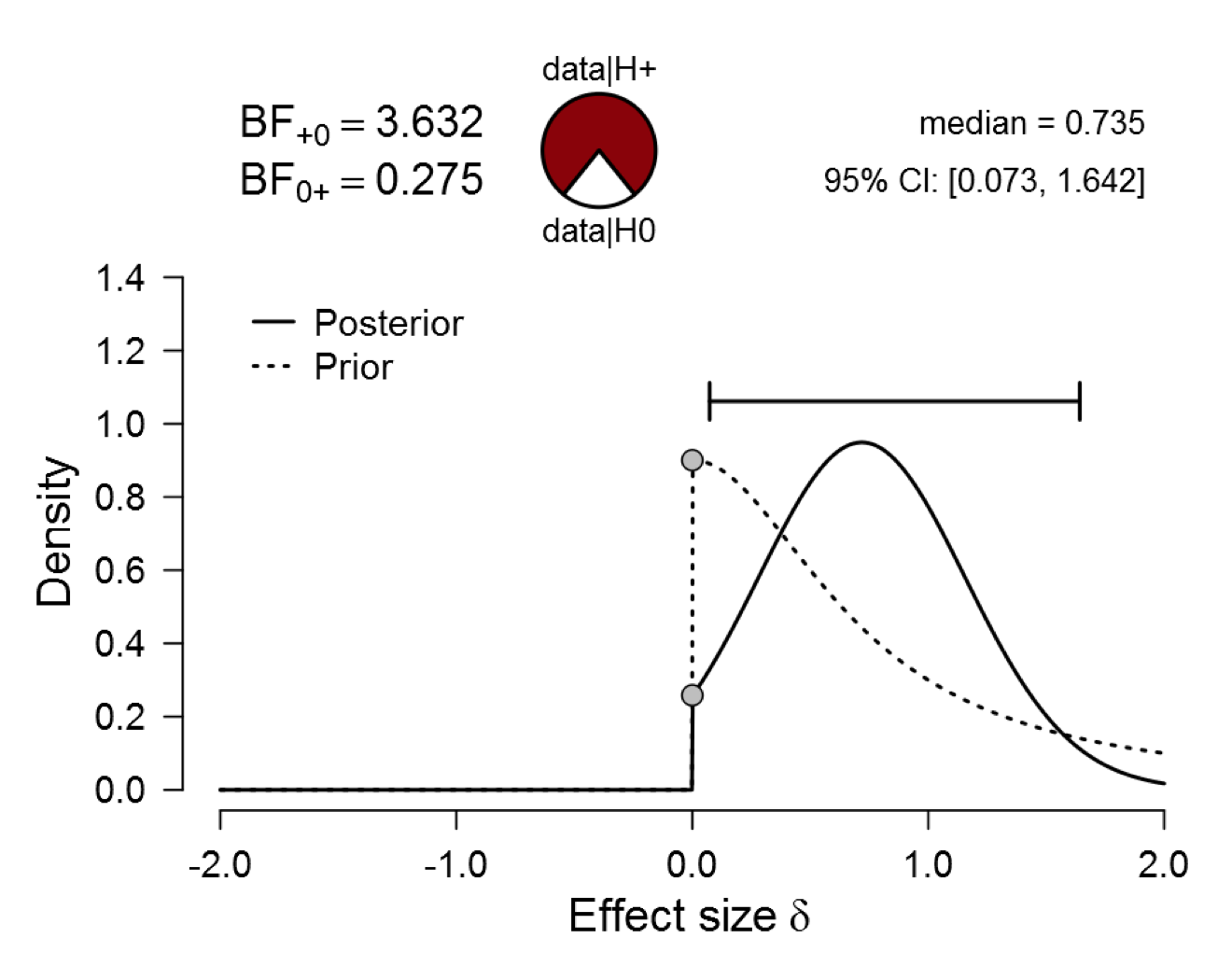
Figure 2. Bayesian reanalysis of data that give t(20) = 2.18, p = .042. The prior under H1 is a one-sided default Cauchy with location 0 and scale 0.707. The evidence for H1 is not compelling. Figure from JASP.
REMARK 3. The posterior distributions from the Oosterwijk prior and the default one-sided prior are very different. Nevertheless, the evidence against the null hypothesis is almost identical. This confirms Remark 1 that the assessment of evidence cannot be based on the posterior distribution alone.
For the present purposes, the main point here is that the Oosterwijk prior does not produce compelling evidence against the null.
What About A Normal Prior Distribution Centered on the Effect Size Obtained?
Recall that the observed effect size was d=.95. We can use the Summary Stats module in JASP to specify a prior distribution that is centered on the observed d. This is statistical cheating, because in the absence of a working crystal ball there is no way to anticipate this value. For this reason, such priors are called “oracle” priors.
First we examine the scenario with a prior centered on .95 but with a standard deviation of .10, meaning that the researcher is 68% sure that the true effect falls in between .85 and 1.05. We regard this as an extremely optimistic and overconfident proposition. The result is as follows:
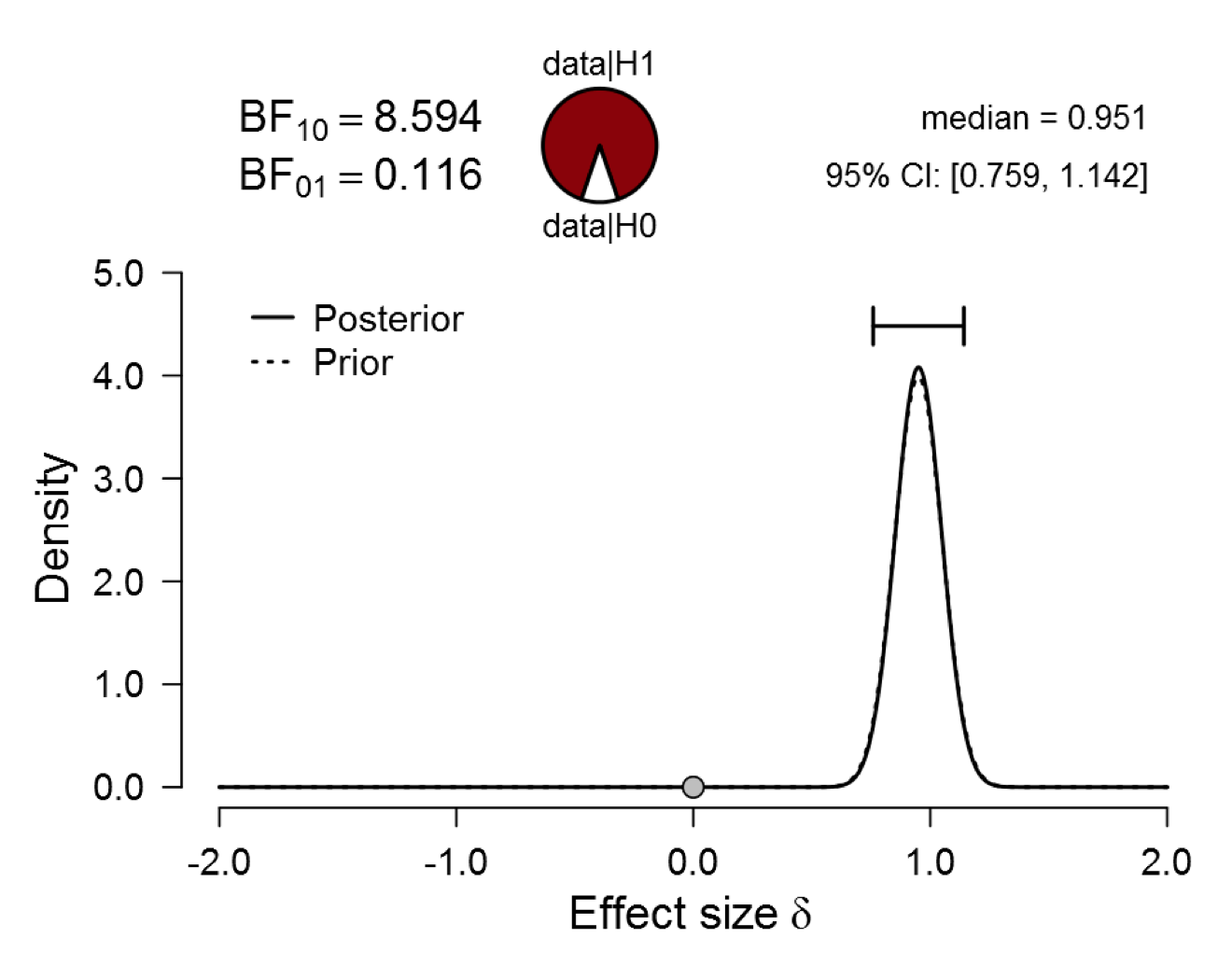
Figure 3. Bayesian reanalysis of data that give t(20) = 2.18, p = .042. The prior under H1 is a Normal distribution with mean 0.95 (i.e., the observed effect size) and standard deviation 0.1. The evidence for H1 is noticeable, but the prior distribution is implausible. Figure from JASP.
REMARK 4. Note that the prior and posterior distributions look almost identical. Nevertheless, the Bayes factor is 8.594, the most compelling evidence we’ve managed to squeeze from the data so far. This paradoxical result occurs because the Bayesian test depends on the prior and posterior ordinate at an effect size of zero (for an explanation see Wagenmakers et al., 2010), that is, an effect in the tails of the distribution. The upshot is that a visual comparison of the prior and posterior distribution is potentially misleading, unless one zooms in on the height of the two distributions at an effect size of zero (something that may be difficult to do when both distributions are away from zero).
Are we happy with a Bayes factor of 8.594? Well, that depends. Firstly, we can look at the pizza plot immediately above the figure and execute a mental PAW (Pizza-poke Assessment of the Weight of evidence): imagine poking a finger blindly into the pepperoni (red area) and mozzarella (white area) pizza; how surprised are you when your finger comes back covered in mozzarella? You would be somewhat surprised, but is it enough to make the all-or-none claim that the effect is present? It seems that it is more prudent to acknowledge the continuous nature of the evidence. Secondly, the Bayesian analysis is one-sided. Consistent with the two-sided nature of the classical analysis, a symmetric Bayesian two-sided analysis would put half of the prior mass near -.95; this effectively halves the Bayes factor, reducing it to about 4. Thirdly, a Bayes factor of 8.594 is still not as strong as a p-value of .042 may suggest (“1-in-20”). Finally, this prior distribution is preposterous, as it requires a crystal ball.
We can obtain the absolute maximum Bayes factor by specifying prior distribution that assigns all mass to the observed effect size, that is, a normal distribution with mean d=.95 and standard deviation 0. This yields a Bayes factor of about 8.8. This absolute maximum is still not as compelling as p=.042 suggests. Over half a century ago, Edwards et al. (1963, p. 228) concluded that “Even the utmost generosity to the alternative hypothesis cannot make the evidence in favor of it as strong as classical significance levels might suggest.”
Take-home Messages
Contrary to popular belief, we have shown by example that an assessment of the evidence against the null hypothesis cannot be obtained by eyeballing the posterior distribution. Identical evidence can be associated with highly dissimilar posterior distributions, and highly dissimilar evidence can be associated with identical posterior distributions. It is more appropriate to eyeball both the prior and the posterior distribution, but even here intuition can be misleading, as the evidence is given by height ratio of the two distributions at the value under test (cf. the last figure above).
Most importantly, we have demonstrated that centering the prior away from zero does not make the key problem with p-values go away. P-values near .05 remain evidentially unconvincing, even if one uses an oracle prior and places all mass on the observed effect, especially when one respects the two-sided nature of the analysis.
One may argue that our demonstration was effective only because sample size in the Elliot et al. study was relatively low. In the next post we will therefore discuss a different example with almost 200 participants.
Like this post?
Subscribe to the JASP newsletter to receive regular updates about JASP including the latest Bayesian Spectacles blog posts! You can unsubscribe at any time.
References
Edwards, W., Lindman, H., & Savage, L. J. (1963). Bayesian statistical inference for psychological research. Psychological Review, 70, 193-242.
Elliot, A. J., Kayser, D. N., Greitemeyer, T., Lichtenfeld, S., Gramzow, R. H., Maier, M. A., Liu, H. (2010). Red, rank, and romance in women viewing men. Journal of Experimental Psychology: General, 139, 399-417.
Gronau, Q. F., Ly, A., & Wagenmakers, E.-J. (2017). Informed Bayesian t-tests. Manuscripts submitted for publication. Available at https://arxiv.org/abs/1704.02479.
JASP Team (2017). JASP (Version 0.8.2) [Computer software]
Ly, A., Raj, A., Marsman, M., Etz, A., & Wagenmakers, E.-J. (2017). Bayesian reanalyses from summary statistics: A guide for academic consumers. Manuscript submitted for publication. Available at https://osf.io/7t2jd/.
Wagenmakers, E.-J., Lodewyckx, T., Kuriyal, H., & Grasman, R. (2010). Bayesian hypothesis testing for psychologists: A tutorial on the Savage-Dickey method. Cognitive Psychology, 60, 158-189.
Wasserstein, R. L., & Lazar, N. A. (2016). The ASA’s Statement on p-values: Context, process, and purpose. The American Statistician, 70, 129-133.
About The Authors

Eric-Jan Wagenmakers
Eric-Jan (EJ) Wagenmakers is professor at the Psychological Methods Group at the University of Amsterdam.

Quentin Gronau
Quentin is a PhD candidate at the Psychological Methods Group of the University of Amsterdam.