Popular Misconceptions About Bayesian Inference: Introduction to a Series of Blog Posts

October 26 - 2017

“By seeking and blundering we learn.”

– Johann Wolfgang von Goethe

Bayesian methods have never been more popular than they are today. In the field of statistics, Bayesian procedures are mainstream, and have been so for at least two decades. Applied fields such as psychology, medicine, economy, and biology are slow to catch up, but in general researchers now view Bayesian methods with sympathy rather than with suspicion (e.g., McGrayne 2011).

The ebb and flow of appreciation for Bayesian procedures can be explained by a single dominant factor: pragmatism. In the early days of statistics, the only Bayesian models that could be applied to data were necessarily simple – the more complex, more interesting, and more appropriate models escaped the mathematically demanding derivations that Bayes’ rule required. This meant that unwary researchers who accepted the Bayesian theoretical outlook effectively painted themselves into a corner as far as practical application was concerned. How convenient then that the Bayesian paradigm was “absolutely disproved” (Peirce 1901, as reprinted in Eisele 1985, p. 748); how reassuring that it would “break down at every point” (Venn 1888, p. 121); and how comforting that it was deemed “utterly unacceptable” (Popper 1959, p. 150).

Figure 1.1: Contrary to popular belief, this is probably not Thomas Bayes (c. 1701-1761). For details see the discusion by Prof. David R. Bellhouse.

All of this changed with the advent of Markov chain Monte Carlo (MCMC; Gilks et al. 1996, van Ravenzwaaij et al. in press), a set of numerical techniques that allows users to replace mathematical so- phistication with raw computing power. Instead of having to derive a posterior distribution, MCMC draws many samples from it, and the resulting histogram approximates the posterior distribution to arbitrary precision (i.e., if you want a more precise approximation, just have the algorithm draw more samples). And it gets better. Probabilistic programming languages such as BUGS (Lunn et al. 2012), JAGS (Plummer 2003), and Stan (Carpenter et al. 2017) circumvent the need to code your own, problem-specific MCMC algorithm; instead, users can specify a complex model in only a few lines. One random example, adorned with comments that follow the hashtag:

# A Bayesian Mixture Model Analysis of the Reproducibility
# Project: Psychology, in 7 lines of code.
### Priors on the Mixture Model Parameters ###
# A vague prior on study precision:
tau ~ dgamma(0.001,0.001)
# A flat prior on the true effect rate:
phi ~ dbeta(1,1)
# A flat prior on slope for predicted effect under H1:
alpha ~ dunif(0,1)
### Mixture Model Likelihood ###
for(i in 1:n){
# Point prediction is mu[i]:
repEffect[i] ~ dnorm(mu[i],tau)
# clust[i] = 0 for H0, clust[i] = 1 for H1
clust[i] ~ dbern(phi)
# when clust[i] = 0, then mu[i] = 0;
# when clust[i] = 1, then mu[i] = alpha * orgEffect[i]:
mu[i] <- alpha * orgEffect[i] * equals(clust[i],1)
}

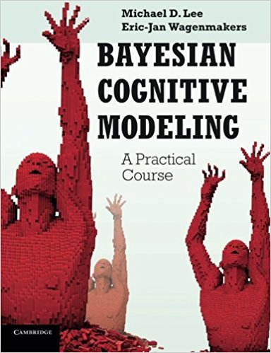Figure 1.2: The cover of Bayesian Cog- nitive Modeling (Lee and Wagenmak- ers 2013), featuring “red” by lego-artist Nathan Sawaya (click here for more examples). With ‘lego-like’ building blocks, Bayesian prob- abilistic programming languages allow the user to create models that respect the complexity of real-world processes.

The specifics of the above model are irrelevant; the model syntax is provided here only to give an impression of how easy it is to define a relatively complex model in a few lines of code. Granted, you have to know which lines of code, but that challenge is on a more conceptual plane. A program like JAGS accepts the model syntax, automatically executes an MCMC algorithm, and then produces samples from the joint posterior. Bayesian magic!

All of the probabilistic programming languages come with a series of hard-wired densities and functions (e.g., dnorm for the density of a normal distribution). These can be thought of as building blocks similar to lego. With these ‘lego blocks’, users can construct models that are limited only by their imagination. MCMC turned the world upside down: suddenly it became evident that, by clinging to their inferential framework, it had been the frequentists, not the Bayesians, who had painted themselves into a pragmatically unenviable corner. Stuck with an awkward philosophy of science and an inflexible set of tools to boot, the decline of frequentist statistics seems inevitable.¹

So here we are. MCMC has unshackled Bayesian inference, and now it roams free, allowing researchers worldwide to update their knowledge, to quantify evidence, and to make predictions by projecting uncertainty into the future. Never before has Bayesian inference been easier to apply, never before has its application met with so much interest and approval.

Figure 1.3: Output from the Donald Trump insult generator. Visit http://time.com/3966291/donald-trump-insult-generator and enter ‘frequentist’ for more thought-provoking observations.

But there are dangers. The ease of practical application may blind novices to the theoretical subtleties of Bayesian inference, causing persistent misinterpretations. And statistical experience need not alleviate the problem: when dyed-in-the-wool frequentists are struggling to get to grips with Bayesian concepts that are alien to them, an initial phase of confusion is often followed by a second phase of misinterpretation. This second stage can sometimes last a lifetime. Bayesian proponents may be tempted to think that fundamental misconceptions are a curse that affects only frequentist statistics, whereas Bayesian concepts are intuitive and straightforward; unfortunately –and despite what the Trump insult generator will tell you about frequentists (‘hokey garbage frequentists’)– that is fake news. We speak from experience when we say that even researchers with a decent background in Bayesian theory can fall prey to misinterpretations. Statistics, it appears, is surprisingly difficult.

For instance, in the blog post ‘The New SPSS Statistics Version 25 Bayesian Procedures’, senior software engineer Jon Peck discussed Bayesian additions to SPSS:

The other interesting statistic is the Bayes Factor, 1.15. It is just the ratio of the data likelihoods given the null versus the alternative hypothesis. So we can say that the alternative hypothesis is 15% more likely than the null. We don’t have a way to make a statement like that using classical methods.” (https://developer.ibm.com/predictiveanalytics/2017/ 08/18/new- spss- statistics- version- 25- bayesian- procedures/)²

Figure 1.4: Dewi Sri, goddess of rice and fertility. By Gunawan Kar- tapranata – Own work, CC BY-SA 3.0, https://commons.wikimedia.org/w/index.php?curid=10253618.

Jon Peck is clearly a smart person with the time and skill to implement Bayesian procedures in one of the world’s most profitable computer programs. Nevertheless, his interpretation of the Bayes factor is incorrect, and not in a subtle way. First, a Bayes factor of 1.15 indicates that the observed data are 1.15 times more likely to occur under H1 than under H0; it most emphatically does not mean that H1 is 1.15 times more likely than H0. In order to make a statement about the (relative) posterior probability of the hypotheses, one needs to take into account their (relative) prior plausibility; H1 could be ‘plants grow faster with access to water and sunlight’, or it could be ‘plants grow faster when you pray for their health to Dewi Sri’. Because the prior plausibility for these hypotheses differs, so will the posterior plausibility, particularly when the observations turn out to be identical and the Bayes factor in both cases equals 1.15.

Second, a Bayes factor of 1.15 does not relate in any way to something like 15%. In fact, a Bayes factor of 1.15 conveys a mere smidgen of evidence. To see this, assume that the H0 and H1 are equally likely a priori, so that p(H1) = 0.50. Upon seeing data that provide a Bayes factor of 1.15, this prior value of 0.50 is updated to a posterior value of 1.15/2.15 ≈ 0.53. Jeffreys (1939, p. 357) called any Bayes factor less than about 3 ‘not worth more than a bare comment’ and that epithet is certainly appropriate in this case.

The goal of this series of blog posts is simple. We wish to provide a comprehensive list of misconceptions concerning Bayesian inference. In order to demonstrate that we are not just making it up as we go along, we have tried to cite the relevant literature for background information, and we have illustrated our points with concrete examples. Some of the misconceptions that we will discuss are our own, and correcting them has deepened our appreciation for the elegance and coherence of the Bayesian paradigm.

We hope the intended blog posts are useful for students, for beginning Bayesians, and for those who have to review Bayesian manuscripts. We also hope the posts will help clear up some of the confusion that inevitably arises whenever Bayesian statistics is discussed online. We imagine that, when confronted with a common Bayesian misconception, one may just link to a post, along the lines of ‘Incorrect. This is misconception #44.’ Doing so will not win popularity contests, but you will be right, and that’s all that matters — in the long run, at least.

Like this post?

Subscribe to the JASP newsletter to receive regular updates about JASP including the latest Bayesian Spectacles blog posts! You can unsubscribe at any time.

Footnotes

¹ We grudgingly admit that there exist some statistical scenarios in which frequentist procedures are relatively flexible.

² The phrase “So we can say that the alter- native hypothesis is 15% more likely than the null.” was later replaced with the phrase “So we can say that the null and alternative hypotheses are about equally likely.” Both phrases are false.

References

Carpenter, B., Gelman, A., Hoffman, M., Lee, D., Goodrich, B., Betancourt, M., Brubaker, M. A., Guo, J., Li, P., & Riddell, A. (2017). Stan: A probabilistic programming language. Journal of Statistical Software, 76.

Eisele, C. (1985). Historical Perspectives on Peirce’s Logic of Science: A History of Science. Berlin: Mouton Publishers.

Gilks, W. R., Richardson, S., & Spiegelhalter, D. J. (1996, Eds.). Markov Chain Monte Carlo in Practice. Boca Raton (FL): Chapman & Hall/CRC.

Jeffreys, H. (1939). Theory of Probability. Oxford: Oxford University Press.

Lee, M. D., & Wagenmakers, E.-J. (2013). Bayesian Cognitive Modeling: A Practical Course. Cambridge: Cambridge University Press. A hands-on book with many examples. The material in this book forms the basis of an annual week-long workshop in Amsterdam (organized in August, directly before or after the JASP workshop).

Lunn, D., Jackson, C., Best, N.,Thomas, A., & Spiegelhalter, D.J. (2012). The BUGS Book: A Practical Introduction to Bayesian Analysis. Boca Raton, FL: Chapman & Hall/CRC.

McGrayne, S. B. (2011). The Theory that Would not Die: How Bayes’ Rule Cracked the Enigma Code, Hunted Down Russian Submarines, and Emerged Triumphant from Two Centuries of Controversy. New Haven, CT: Yale University Press.

Plummer, M. (2003). JAGS: A program for analysis of Bayesian graphical models using Gibbs sampling. In Hornik, K., Leisch, F., & Zeileis, A. (eds.), Proceedings of the 3rd International Workshop on Distributed Statistical Computing. Vienna, Austria.

Popper, K. R. (1959). The Logic of Scientific Discovery. New York: Harper Torchbooks.

van Ravenzwaaij, D., Cassey, P., & Brown, S. D. (in press). A simple in- troduction to Markov chain Monte-Carlo sampling. Psychonomic Bulletin & Review.

Venn, J. (1888). The Logic of Chance (3rd ed.). New York: MacMillan.