
This post is inspired by Morey et al. (2016), Rouder and Morey (in press), and Wagenmakers et al. (2016a).
The Misconception
Bayes factors may be relevant for model selection, but are irrelevant for
parameter estimation.
The Correction
For a continuous parameter, Bayesian estimation involves the computation of an infinite number of Bayes factors against a continuous range of different point-null hypotheses.
The Explanation
Let H0 specify a general law, such that, for instance, the parameter θ has a fixed value θ0. Let H1 relax the general law and assign θ a prior distribution p(θ | H1). After acquiring new data one may update the plausibility for H1 versus H0 by applying Bayes’ rule (Wrinch and Jeffreys 1921, p. 387):
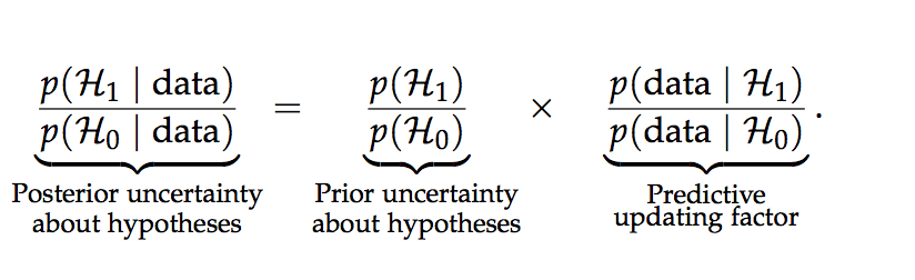
This equation shows that the change from prior to posterior odds is brought about by a predictive updating factor that is commonly known as the Bayes factor (e.g., Etz and Wagenmakers 2017). The Bayes factor pits the average predictive adequacy of H1 against that of H0.
Some statisticians, however, are uncomfortable with Bayes factors. Their discomfort is usually due to two reasons: (1) the fact that some Bayes factors involve a point-null hypothesis H0, which is deemed implausible or uninteresting on a priori grounds; (2) the fact that Bayes factors depend on the prior distribution for the model parameters. Specifically, p(data | H1) can be written as ∫Θ p(data | θ, H1)p(θ | H1) dθ, from which it is seen that the marginal likelihood is an average value for p(data | θ, H1) across the parameter space, with the averaging weights provided by the prior distribution p(θ | H1). It is commonly assumed that the discomfort with Bayes factors can be overcome by focusing on parameter estimation, that is, ignoring the point-null H0 altogether and deriving the posterior distribution under the alternative hypothesis, that is, p(θ | data, H1).
It may then come as a surprise that, for a continuous parameter θ, the act of estimation involves the calculation of an infinite number of Bayes factors against a continuous range of point-null hypotheses. To see this, write Bayes’ rule as follows (now suppressing the conditioning on H1):
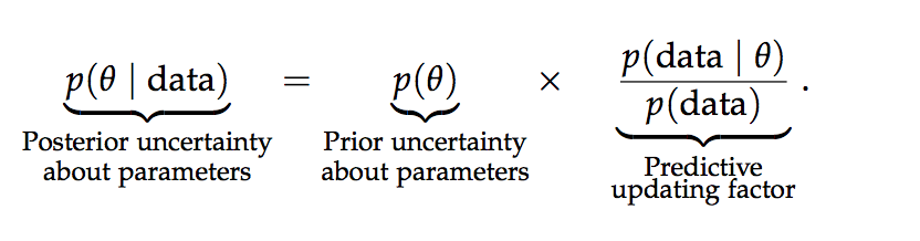
This equation shows that the change from the prior to the posterior distribution of θ is brought about by a predictive updating factor. This factor considers, for every parameter value θ, its success in probabilistically predicting the observed data – that is, p(data | θ) – as compared to the average probabilistic predictive success across all values of θ – that is, p(data).The fact that p(data) is the average predictive success can be appreciated by rewriting it as ∫Θ p(data | θ)p(θ)dθ. In other words, values of θ that predict the data better than average receive a boost in plausibility, whereas values of θ that predict the data worse than average suffer a decline (Wagenmakers et al. 2016a).
But for any specific value of θ, this predictive updating factor is simply a Bayes factor against a point-null hypothesis H0 : θ = θ0. For a continuous prior distribution then, the updating process requires the computation of an infinity of Bayes factors. Note that multiplicity is punished automatically because the prior distribution is spread out across the various options (i.e., the different values of θ). The relation between Bayesian parameter estimation and testing a point- null hypothesis is visualized in Figure 1.
The predictive updating factor from Equation 2 has been discussed earlier by Carnap (1950, pp. 326-333), who called it “the relevance quotient” (Figure 2). Still earlier, the predictive updating factor was discussed by Keynes (1921), who called it the “coefficient of influence” (p. 170; as acknowledged by Carnap). Keynes, in turn, may have been influenced by W. E. Johnson.
In sum, the Bayes factor is the epistemic engine in Bayes’ rule, and it plays a vital role both in model selection and parameter estimation.
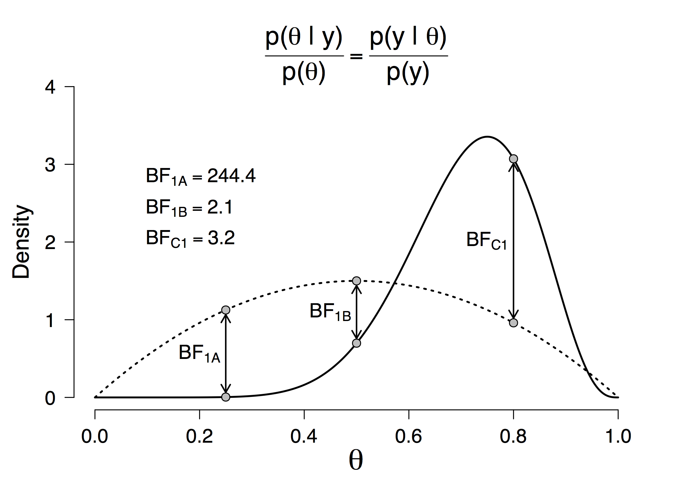
Figure 1: In Bayesian parameter esti- mation, the plausibility update for a specific value of θ (e.g., θ0) is mathematically identical to a Bayes factor against a point-null hypothesis H0 : θ = θ0. Note the similarity to the Savage-Dickey density ratio test (e.g., Dickey and Lientz 1970, Wetzels et al. 2010).
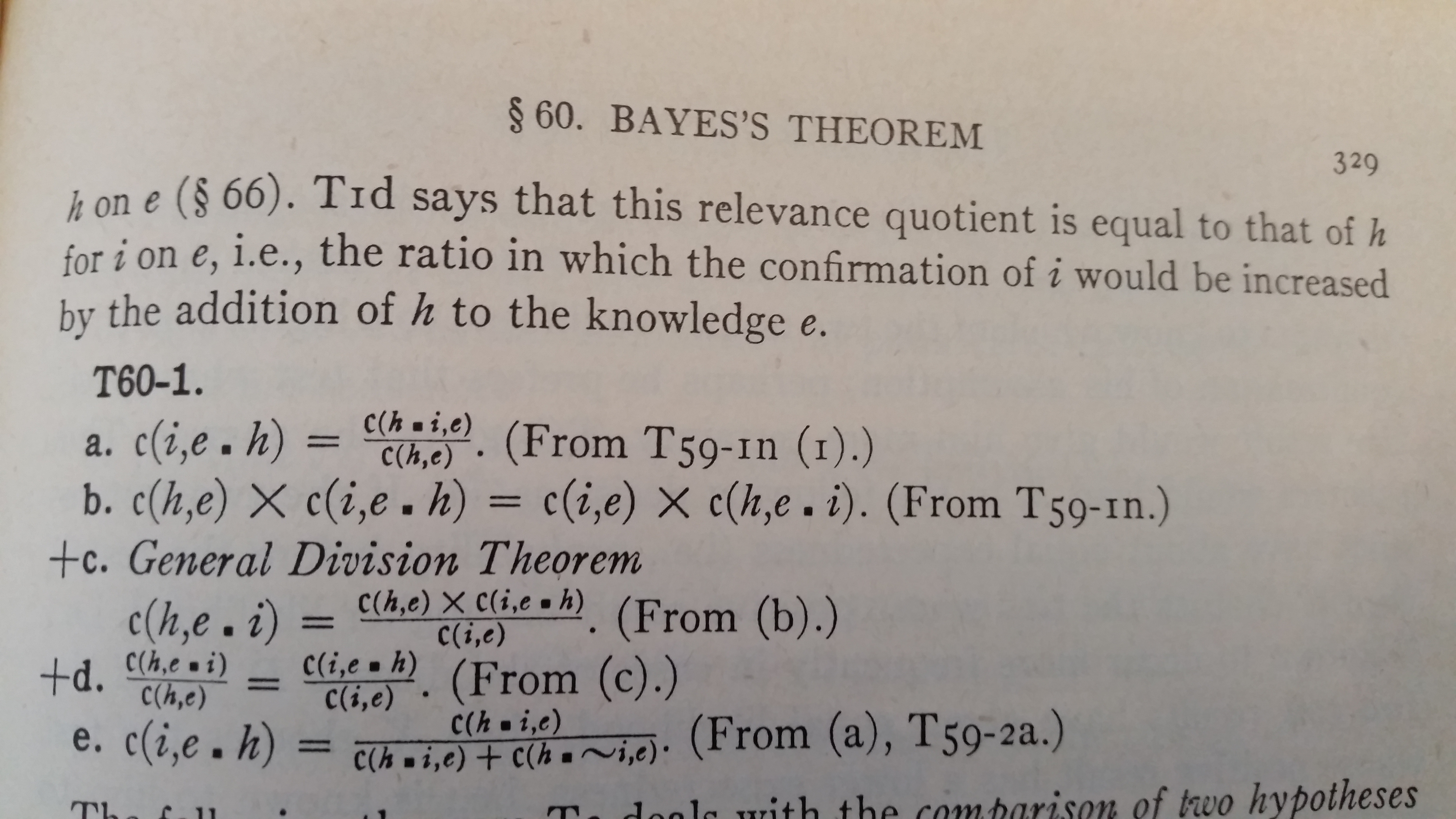
Figure 2: On page 329 of “Logical Foundations of Probability”, Carnap explicitly discusses the predictive updating factor, which he called the relevance quotient.
Like this post?
Subscribe to the JASP newsletter to receive regular updates about JASP including the latest Bayesian Spectacles blog posts! You can unsubscribe at any time.
References
Carnap, R. (1950). Logical Foundations of Probability. Chicago: The University of Chicago Press.
Dickey, J. M., & Lientz, B. P. (1970). The weighted likelihood ratio, sharp hypotheses about chances, the order of a Markov chain. The Annals of Mathematical Statistics, 41, 214-226.
Keynes, J. M. (1921). A Treatise on Probability. London: Macmillan & Co.
Etz, A., & Wagenmakers, E.–J. (2017). J. B. S. Haldane’s contribution to the
Bayes factor hypothesis test. Statistical Science, 32, 313-329.
Morey, R. D., Romeijn, J. W., & Rouder, J. N. (2016). The philosophy of Bayes factors and the quantification of statistical evidence. Journal of Mathematical Psychology, 72, 6-18.
Rouder, J. N., & Morey, R. D. (in press). Teaching Bayes’ theorem: Strength of evidence as predictive accuracy. The American Statistician.
Wagenmakers, E.–J., Morey, R. D., & Lee, M. D. (2016). Bayesian benefits for the pragmatic researcher. Current Directions in Psychological Science, 25, 169-176.
Wetzels, R., Grasman, R. P. P. P., & Wagenmakers, E.–J. (2010). An encompassing prior generalization of the Savage–Dickey density ratio test. Computational Statistics & Data Analysis, 54, 2094-2102.
About The Authors

Eric-Jan Wagenmakers
Eric-Jan (EJ) Wagenmakers is professor at the Psychological Methods Group at the University of Amsterdam.

Quentin Gronau
Quentin is a PhD candidate at the Psychological Methods Group of the University of Amsterdam.