In the previous post I asked the following question:

Here is a test of your Bayesian intuition: Suppose you assign a binomial chance parameter θ a beta(2,2) prior distribution. You anticipate collecting two observations. What is your expected posterior distribution?

NB. ChatGPT 3.5, Bard, and the majority of my fellow Bayesians get this wrong. The answer will be revealed in the next post.

The incorrect answer often goes a little something like this: under a beta(2,2) prior for θ, the expected number of successes equals 1 (and hence the expected number of failures also equals 1). Hence, the expected posterior ought to be a beta(3,3) distribution; feeling that this was not quite correct, some Bayesians guessed a beta(2.5,2.5) distribution instead. (note that updating a beta(2,2) distribution with s successes and f failures results in a beta(2+s,2+f) posterior)

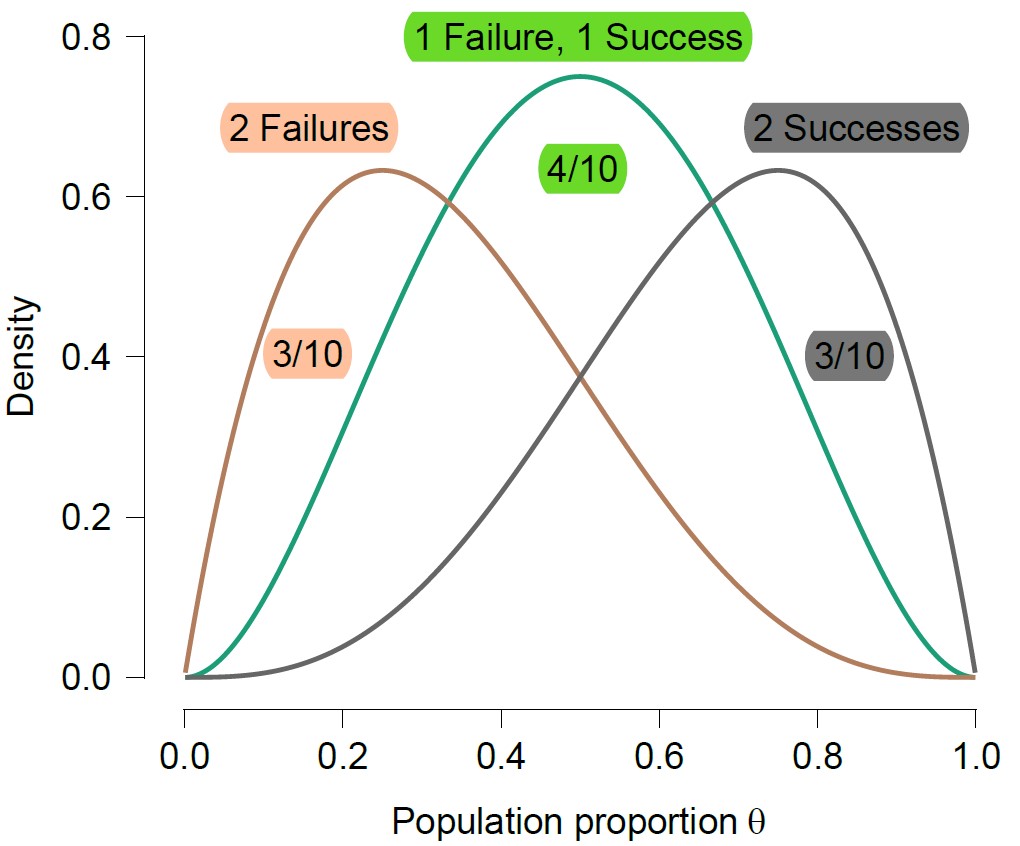
To arrive at the correct answer, let’s take this one step at a time. First of all, there are three possible outcomes that may arise: (a) two successes; (b) two failures, and (c) a combo of one success and one failure. If case (a) arises, we have a beta(4,2) posterior; of case (b) arises, we have a beta(2,4) posterior; and if case (c) arises, we have a beta(3,3) posterior. Hence, our expected posterior is a mixture of three beta distributions. The mixture weights are given by the probabilities for the different cases. These probabilities can be obtained from the beta-binomial distribution — the probability for both scenario (a) and scenario (b) is 3/10, with scenario (c) collecting the remaining 4/10. The three component mixture is displayed below:

The mixture interpretation is spot-on, but the desired answer is considerably simpler. The correct intuition is that the anticipation about future observations is a kind of prior predictive. With the model and the prior distribution for θ already in place, the prior predictive adds no novel information whatsoever. The mere act of entertaining future possibilities does not alter one’s epistemic state concerning θ one iota. Hence, the expected posterior distribution simply equals the prior distribution — in our case then, the expected posterior distribution is just the beta(2,2) prior distribution!

This “law” is known as the reflection principle (ht to Jan-Willem Romeijn) and related to martingale theory. I may have more to say about that at some later point. Some references include Goldstein (1983), Skyrms (1997), and Huttegger (2017). Of course, when you have the right intuition the result makes complete sense and is not surprising; nevertheless, I find it extremely elegant. Note, for instance, that the regularity holds regardless of how deep we look into the future. Consider for instance a hypothetical future data set of 100 observations. This yields 101 different outcomes (we have to count the option of zero successes); in this case the expected posterior distribution is still the beta(2,2) prior distribution, but now it is a 101-component beta mixture, with the 101 weights set exactly so as to reproduce the beta(2,2) prior. Another immediate insight is based on the Bayesian central limit theorem, which states that under regularity conditions, all posterior distribution become normally distributed around the MLE, no matter the shape of the prior distribution. From this one can infer that all prior distributions, no matter their shape, can be well approximated by a finite mixture of normals (i.e., take any prior distribution. Then imagine a very large sample size such that the resulting posterior distributions are all approximately normal. The prior distribution is a mixture of these approximate normals. QED)

As Erik-Jan van Kesteren pointed out on Mastodon, it is a little strange to speak of “expectations”. When we entertain 100 additional observations, say, we know for a fact that any resulting posterior will be much more narrow than the beta(2,2) prior. Hence the beta(2,2) is not representative for any single posterior distribution that may obtain. It may therefore be more intuitive to speak of an “average” posterior probability. As is often forgotten, the average need not be representative of any particular unit that is included in the average.

For Unbelievers

For those who do not want to take my word for it, here is a simple derivation:

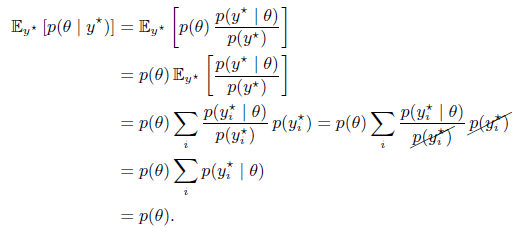
In the above equation, the final sum evaluates to 1 because it is the total probability across all possible data.

Those who do not put their trust in mathematics may convince themselves by trying out the analysis in JASP. In the Binomial Testing procedure of the Learn Bayes module, the beta mixture components can be specified as follows:

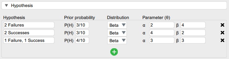
The resulting prior mixture can be examined either as the “joint” (which shows the individual components) or as the “marginal” (which produces the typical dome-like beta(2,2) shape).

Coherence, Coherence, Coherence

The elegant answer to the question is yet another consequence of coherence. Throughout his career Dennis Lindley stressed the importance of coherence and famously stated that “today’s posterior is tomorrow’s prior” (Lindley 1972, p. 2). The result here can be summarized by stating that “today’s prior is our expectation for tomorrow’s posterior“. As an aside, Lindley also tried to promote the term “coherent statistics” as a replacement for the more obscure “Bayesian statistics”. Unfortunately that horse has bolted several decades ago, but it was a good idea nevertheless.

References

Huttegger, S. M. (2017). The probabilistic foundations of rational learning. Cambridge: Cambridge University Press.

Skyrms, B. (1997). The structure of radical probabilism. Erkenntnis, 45, 285-297.

Goldstein, M. (1983). The prevision of a prevision. Journal of the American Statistical Association, 78, 817-819.

Lindley, D. V. (1972). Bayesian statistics, a review. Philadelphia, PA: SIAM.