Image by Doremi/Shutterstock.com

TLDR; The Last Dance

This post demonstrates how Bayes factors are coherent in the sense that the same result obtains regardless of whether the data are analyzed all at once, in batches, or one at a time. The key point is that this coherence arises because Bayes factors are relatively sensitive to the prior distribution.

Ironically, the sensitivity of the Bayes factor to the shape of the prior distribution has often been viewed as its Achilles’ heel, and many Bayesians have proposed alternative model selection methods to overcome this perceived limitation. However reasonable, well-intentioned, and technically sophisticated these proposals may appear to be, they all suffer the same fate: by achieving their stated goal –robustness to the prior distribution– the resulting methods are doomed to be incoherent (harsh synonyms: internally inconsistent, preposterous, silly, ridiculous, ludicrous, absurd, farcical, foolish). Instead of an Achilles’ heel, the dependence of the Bayes factor on the prior distribution constitutes a necessary condition for coherence.

Those who wish to remove the garlic necklace of prior influence should seriously reconsider, for their next dance partner is likely to be Lord Ludicrus, the vampire Count of Incoherence.

The Sin of Incoherence

In the field of Bayes statistics, incoherence is a cardinal sin; a person who is incoherent issues statements that are internally consistent. For instance, you may state “the probability that the Dutch national men’s soccer team wins the next World Cup is 60%”. This is preposterously high, but it is not necessarily incoherent. It only becomes incoherent when you state, at the same point in time, “the probability that the Dutch national men’s soccer team does not win the next World Cup is 70%” (or indeed any percentage other than 100-60=40%).

Issuing incoherent statements reveals that something epistemically has gone badly off the rails. Supposedly, people who are confronted with the fact that their statements are incoherent will recognize that such statements are not acceptable and will attempt to revise their statements to remove the inconsistency. Incoherence is like the putrid scent of rotten meat; it is not the scent itself that is the main problem; instead, the scent signals that something is wrong with the meat, and it may be best to avoid it.

Although objective Bayesians may argue that certain mild forms of incoherence are an acceptable sacrifice to make in order to be able to specify default prior distributions with desirable properties, militant subjective Bayesians will insist that incoherence is just a fancy word for ludicrous. It is always difficult to win an argument with a subjective Bayesian, and I suspect this is because subjective Bayesians are essentially correct.

Demonstration of Bayes Factor Coherence

The demonstration below is entirely general, and works for any continuous prior distribution and any division of the data into batches. The specific numbers were chosen merely for convenience and to highlight the key message.

We start with the cover story, a fictitious data set, and the standard Bayes factor inference. Consider a matched pairs design to study the effectiveness of chiropractic treatment against neck pain. Specifically, patients are first assigned to pairs based on self-reported intensity of neck pain; in other words, both patients in a pair report about the same intensity of pre-treatment neck pain. Next, one patient from each pair receives a chiropractic treatment, whereas the other patient receives a sham treatment. Of interest is , the population proportion of pairs for which the patient who received the chiropractic treatment reported less neck pain than the patient who underwent the sham-treatment.

In this fictitious setup, we define as the null hypothesis which holds that chiropractic treatment and sham treatment do not differ. For illustrative purposes, the alternative hypothesis is defined as — a uniform distribution that deems every value of equally plausible a priori. Note that according to this prior distribution, the chiropractic treatment may also be harmful (i.e., when ).

The fictitious data show that out of 10 patient pairs, 5 signaled a benefit from the chiropractic treatment (we call these “successes”) and 5 signaled a benefit from the sham treatment (we call these “failures”). In other words, the data show an even split, and this has to mean that the data support over . A few mouse clicks and keystrokes in the Summary Statistics module of JASP yield the following result:

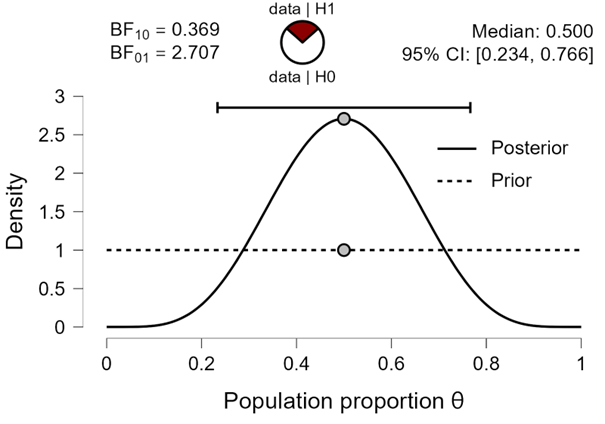
Figure 1. Inference for a population proportion based on the entire data set consisting of 5 successes out of 10 attempts. Figure from JASP.

Figure 1 confirms that the data support middle values of , and the Bayes factor indicates that the observed data are about 2.71 times more likely to occur under than under .

Now we divide the data set in batches A and B. We first do inference on batch A, and then we update our beliefs with the data from batch B. Because Bayes factors are coherent, the result should be exactly the same: 2.71 in favor of . We can divide the data set into two batches any way we like, and this will always work. To stress our key point, we assume that batch A consists of 5 successes and 0 failures, and batch B consequently consists of 0 successes and 5 failures.

First we analyze the data from batch A. With 5 successes and 0 failures, this is the most extreme result possible and one would therefore expect this to yield evidence against . A minimum effort in JASP confirms this intuition:

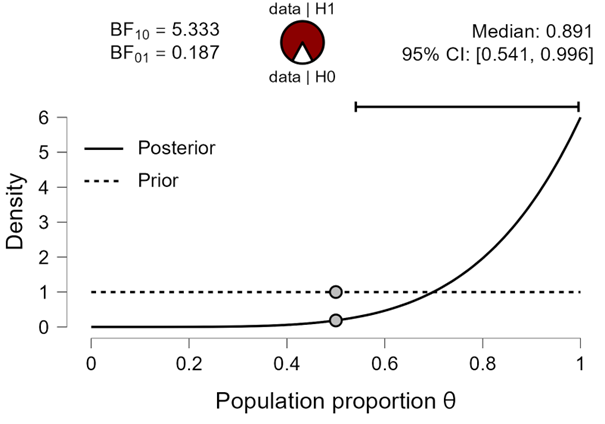
Figure 2. Inference for a population proportion based on batch A, consisting of 5 successes out of 5 attempts. Figure from JASP.

Specifically, the Bayes factor indicates that the data are about 5.33 times more likely to occur under than under . The posterior distribution after batch A has almost all of its mass allocated to values of larger than ½.

We now wish to obtain the Bayes factor for batch B, given our knowledge derived from batch A. Coherence and the law of conditional probability already provide the answer: the Bayes factor for the total data set is 2.71 in favor of , whereas the Bayes factor for batch A is 5.33 in favor of . It must therefore be the case that the Bayes factor for batch B is strong evidence in favor of : it needs to undo the 5.33 push in the wrong direction and then add some additional evidence in order to arrive at the desired 2.71 in favor of . Specifically, the Bayes factor for batch B should be 2.71 * 5.33 ≈ 14.44 in favor of . Note that this desired result is dramatically different from what would obtain if the data from batch A were ignored; in this case we would start the analysis of batch B afresh, with a uniform distribution, and conclude that the data (i.e., 0 successes and 5 failures) are 5.33 times more likely under than under . This would leave us with two batches, each of which signals evidence against , when we know that the complete data set in fact yields evidence in favor of . This would be incoherent.

In order to conduct the coherent analysis, it is crucial to realize that the correct prior distribution for batch B is the posterior distribution obtained from batch A. We started with a uniform beta(1,1) distribution, and after 5 successes and zero failures from batch A this yields the beta(6,1) posterior distribution shown in Figure 2. We then use this beta(6,1) distribution for the analysis of the batch B data. Again, minimal effort in JASP yields the following outcome:

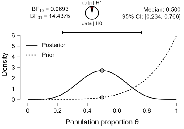
Figure 3. Inference for a population proportion based on batch B, consisting of 0 successes out of 5 attempts. Note that the prior distribution equals the posterior distribution from batch A, and the posterior distribution equals the posterior distribution from the analysis of the complete data set. Figure from JASP.

It is immediately evident that we obtain the coherent answer: the Bayes factor in favor of is about 14.44. Now consider why the batch B analysis is coherent. First, it is clear that any coherent analysis must be able to quantify evidence in favor of , and that this evidence cannot have a bound. Specifically, suppose that (i.e., half of the attempts are successful) and that batch A contains only the successes and batch B only the failures. As grows, the Bayes factor for batch A indicates ever stronger evidence against , an evidential move in the wrong direction which the Bayes factor for batch B needs to overcome.

Second, the reason why the Bayes factor for batch B supports is because of the poor predictive performance of – and this predictive performance is dictated by the prior distribution. Specifically, the beta(6,1) prior encodes the strong expectation that mostly successes will be observed. The data from batch B, however, show the opposite. In other words, under a beta(6,1) prior distribution the occurrence of 0 successes and 5 failures is highly surprising; in fact, these data are about 14.44 times more surprising than they are under . To underscore this point, the Learn Bayes module in JASP allows one to obtain the predictive distribution for the outcome of 5 trials based on a beta(6,1) distribution:

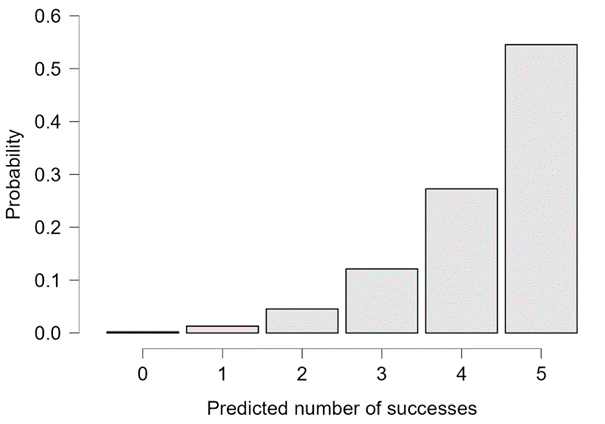
Figure 4. Predictive number of successes out of 5 attempts based on a beta(6,1) distribution. The occurrence of 0 successes out of 5 attempts is highly unlikely. Figure from JASP.

The probability of observing the batch B data (i.e., 0 successes) under a beta(6,1) prior is about .0022; in contrast, the probability of observing these data under is about .0313. For completeness, Figure 5 shows the predictions from .

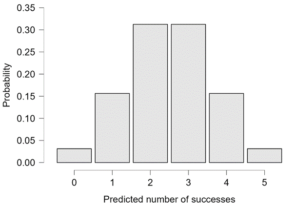
Figure 5. Predictive number of successes out of 5 attempts based on . The occurrence of 0 successes out of 5 attempts is unlikely, but much more likely than it is under the beta(6,1) prior from Figure 4. Figure from JASP.

The main message is that coherence is achieved because the Bayes factor is sensitive to the prior distribution. This sensitivity should be feared nor bemoaned; it is neither too much nor too little – it is exactly what is needed to achieve coherence.

Wrapping Up

Bayes factors are coherent in the sense that the same result obtains irrespective of whether the data arrive all at once, batch-by-batch, or one observation at a time. This is a general property of Bayesian inference that also holds for Bayesian parameter estimation, and it is dictated by the law of conditional probability – therefore it lies at the heart of Bayesian inference.

On a more detailed level, the engine that drives the coherence is the continual adjustment of the prior distribution as the data accumulate. The prior distribution encodes knowledge from the past and allows predictions about the future. As the example from this post demonstrates, the data from batch B needed to provide strong evidence in favor of in order to achieve coherence, and this evidence was produced because the posterior distribution after batch A (i.e., the prior distribution for batch B) yielded predictions that were dramatically wrong. Thus, the reasonable-sounding complaint “but the Bayes factor is sensitive to the shape of the prior distribution” is awfully close to the evidently unreasonable complaint “but the Bayes factor is coherent, and instead we prefer a method that is internally inconsistent”.

Coherence may be taken for granted only by Bayesians who stick to Bayes’ rule religiously. Ad-hoc additions and changes, however reasonable at first sight, are likely to introduce internal inconsistencies. Such incoherence is perhaps Nature’s punishment for tinkering with perfection. I conclude that Bayes factors are coherent, and that this coherence is achieved by the fact that the prior distribution plays a pivotal role in quantifying the old and predicting the new. I speculate that other methods of model selection are either isomorphic to the Bayes factor, or incoherent.

References

Ly, A., Etz, A., Marsman, M., & Wagenmakers, E.-J. (2019). Replication Bayes factors from evidence updating. Behavior Research Methods, 51, 2498-2508.

This study exploits the sequential coherence outlined in this post to quantify replication success; the original study takes the role of batch A, the replication study takes the role of batch B, and replication success is quantified by . The posterior distribution from the original study represents the idealized position of a proponent and acts as the prior distribution for the analysis of the replication study (see also Verhagen & Wagenmakers, 2014).

Jeffreys, H. (1938). Significance tests when several degrees of freedom arise simultaneously. Proceedings of the Royal Society of London. Series A, Mathematical and Physical Sciences, 165, 161-198.

The original source for the central idea of this blog post, as referenced in Ly et al. “Thus it does not matter in what order we introduce our data; as long as we start with the same data and finish with the same additional data, the final results will be the same. The principle of inverse probability cannot lead to inconsistencies.” (Jeffreys, 1938, pp. 191-192)

About The Authors