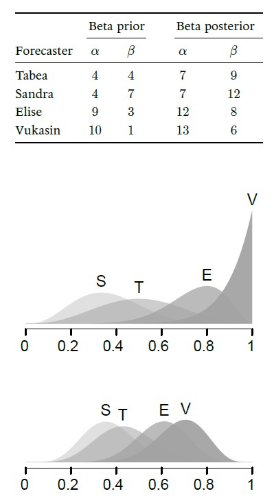
In my research master course “Bayesian Inference for Psychological Science” (co-taught with Dora Matzke), students are asked to specify a beta distribution on the probability θ that I will bake a bacon pancake rather than a standard “vanilla” pancake. So θ is my “bacon proclivity” that students are unsure about. The chapter “The pancake puzzle” from our free course book discusses the results from four pancake forecasters: Tabea, Sandra, Elise, and Vukasin. The chapter first presents their individual beta prior distributions, and then, after observing 3 bacon pancakes and 5 vanilla pancakes, it presents the associated posterior distributions:
 As usual, the data act to bring the initially divergent beliefs closer together. Later in the chapter we discuss how to make a prediction on whether or not the ninth pancake will have bacon. The essential mechanism is to average across the individual forecasters, weighting their individual predictions by their posterior probability. The associated tree diagram shows the law of total probability in action:
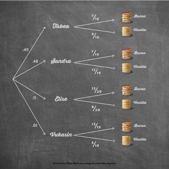
In this tree, the split at the root reflects the posterior probability (NB. at the outset, each forecaster was assigned a prior probability of 1/4). Vukasin and Elise predicted the identity of the first eight pancakes relatively poorly, and this is why less weight is assigned to their predictions compared to those of Tabea and Sandra. The second split is based on averaging over each forecaster’s posterior distribution for my bacon proclivity θ.
Recently it hit me that a very similar averaging operation may be used to obtain the marginal prior and marginal posterior distribution for θ. As dictated by the law of total probability, the marginal prior distribution looks like this:
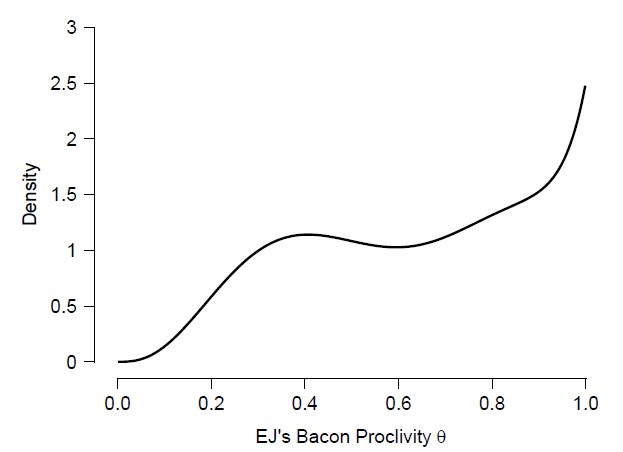
This funky prior distribution reflects the beliefs about θ that is entertained by all forecasters combined: it is a four-component mixture distribution, with the prior probability for each forecaster (i.e., 1/4) functioning as the averaging weight. After observing the data (3 bacon pancakes and 5 vanilla pancakes) the resulting mixture posterior distribution looks like this:
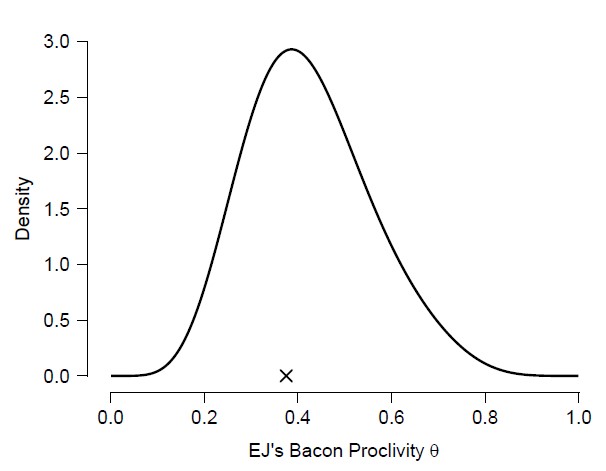
It is noteworthy that the mixture posterior is smooth and unimodal; is it somewhat bell-shaped, but its right tail still bears witness to the mixture prior distribution whence it came. The cross denotes the sample proportion (which is also the maximum likelihood estimate or MLE). According to the Bayesian central limit / Bernstein-von Mises theorem, posterior distributions ought to become bell-shaped (Gaussian) around the MLE when sample size increases (under regularity conditions). We can explore this by increasing the data tenfold; that is, we imagine having observed 30 bacon pancakes and 50 vanilla pancakes. The resulting posterior distribution looks like this:
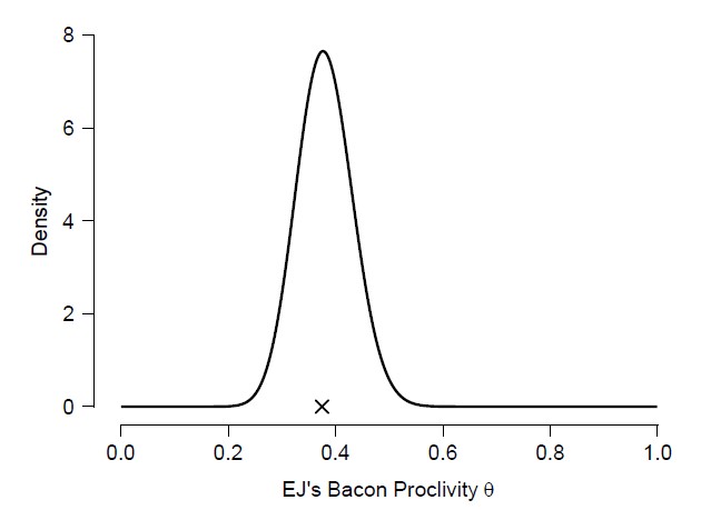
In line with the theorem, the additional data have made the posterior more symmetric around the MLE (and they have of course also decreased the posterior standard deviation). It was interesting to me that the prior mixture distribution takes on such a funky shape, and that a few observations suffice to remove that funkiness completely.
References
Wagenmakers, E.-J., & Matzke, D. (2023). Bayesian inference from the ground up: The theory of common sense.