Inspired by a recent article on Ockham’s razor, this post shows how a simple set of polyhedral dice can clarify the basic idea underlying Bayes factors (or likelihood ratios). The ideas may be used in a classroom demonstration, and each of the lessons below could be discovered by the students themselves.
Meet the Family
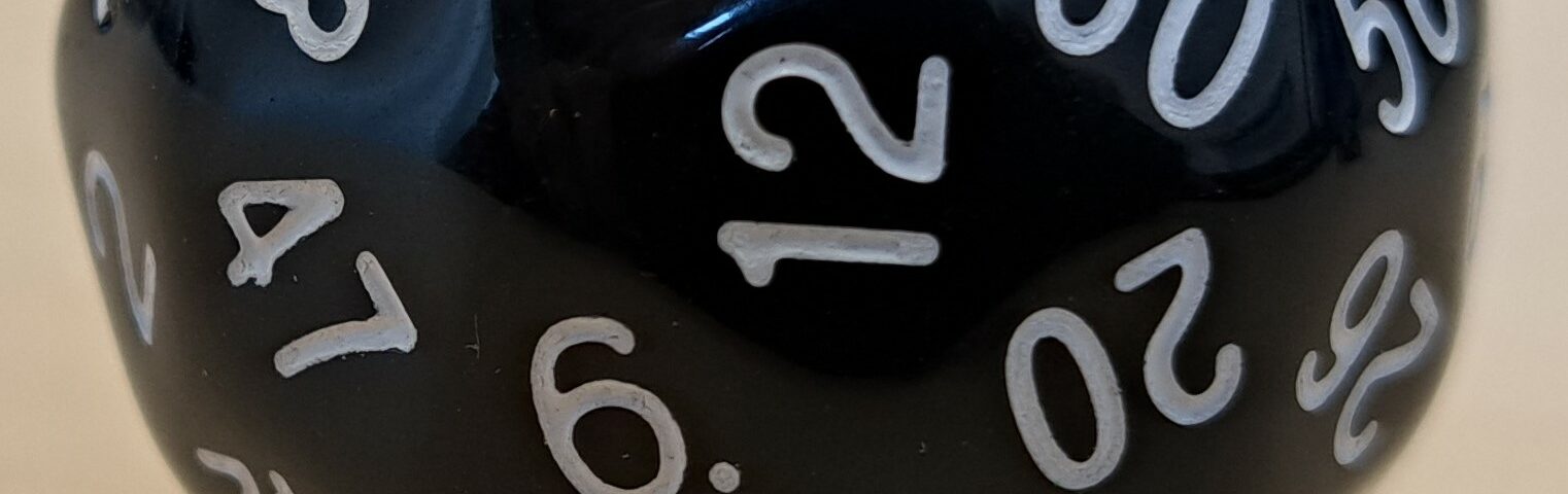
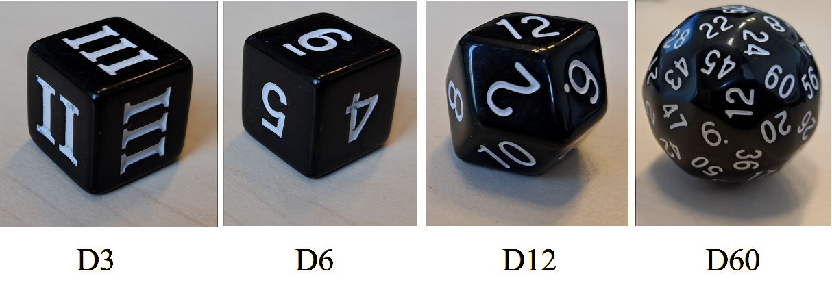
Our polyhedral dice are a family of four. Below you see the D3, the D6 (this is the common six-sided die), the D12, and the D60.
The Setup
You may assume each die is fair. I will first toss the D3 in order to select either the D6, the D12, or the D60. (if the D3 lands “I”, I will select the D6; if the D3 lands “II”, I will select the D12; and if the D3 lands “III”, I will select the D60). Having selected one of the three die, I toss it and report to you only the outcome(s). It is your job to quantify and monitor the evidence, that is, the degree to which the data support the three rival hypotheses (i.e., D6, D12, or D60).
Lesson 1: Ockham’s Razor
Suppose the outcome of the toss is “50”. This outcome is only possible under the D60, and the hypotheses that the die is either the D6 or the D12 are “irrevocably exploded” (Polya). Here we focus on the more interesting case, which is an outcome that is possible under each of the hypotheses. Forget the outcome “50” and instead let’s say we observe the outome “5”. Most people will intuit that this outcome provides evidence in favor of the D6. They may even be able to articulate why: the probability of seeing the outcome is 1/6 under the D6, but 1/12 under the D12, and 1/60 under the D60. The more sides a die has, the more thinly it has to distribute its predictions over the possible outcomes. In other words, D6 is rewarded for making precise, risky predictions that come true. This is exactly the principle that underlies the Bayes factor.
Specifically, the Bayes factor for D6 over D12 is 2 (i.e., (1/6)/(1/12) = 12/6) and the Bayes factor for D6 over D60 is 10 (i.e., (1/6)/(1/60) = 60/6). In words, the observed outcome is twice as likely under D6 than under D12, and ten times as likely under D6 than under D60. In general, suppose the simple die has k1 sides, and the more complex die has k2>k1 sides. An outcome possible under both die will then result in a Bayes factor equal to (k2/k1). If we toss the die a second time, the same computation holds (because we know the die are fair, there are no parameters that need to be updated); if the second outcome is again consistent with both die, the Bayes factor is (k2/k1)^2. After n throws, all of whose outcomes are consistent with both die, the Bayes factor equals (k2/k1)^n.
Lesson 2: Evidence is Relative
Suppose the D3 landed “I” and the selected die is the D6. However, suppose you are unaware that the D6 is in the set. You limit your attention to the Bayes factor for D12 versus D60. On any throw (from the D6 — unbeknownst to you) the outcome will be consistent with both die, but it will be more likely to occur under the D12 than under the D60. Specifically, the Bayes factor for the D12 over the D60 is (1/12)/(1/60) = 60/12 = 5. Now suppose you see the outcome of 10 throws (e.g., 5, 6, 6, 6, 1, 1, 3, 1, 2, 4). The Bayes factor for the D12 over the D60 is then 5^10 = 9,765,625: the data are almost 10 million times more likely under D12 than under D60. But this evidence is relative: the D12 has predicted the outcomes much better than the D60, but that does not mean that we ought to believe that the data actually came from D12. In fact, if we were to learn that the D6 was a possibility, the Bayes factor in its favor over the D12 would be 2^10 = 1024: overwhelming evidence. We can only test hypotheses that we are aware of and deem sufficiently plausible and relevant. When one model outpredicts the other this does not mean that it is close to the “truth”, or that it does well in some absolute sense. The world of probabilities is relative.
Lesson 3: Evidence is Transitive
From the preceding examples it may already be evident that the Bayes factors are transitive. If we know that the Bayes factor for D6 over D12 is 2, and the Bayes factor for D6 over D60 is 10, then it follows that the Bayes factor for D12 over D60 must be 5. For a set of three models, two different Bayes factors suffice to determine the third.
Lesson 4: Gauging the Strength of Evidence
The dice may be used to help researchers appreciate and intuit the strength of evidence that a Bayes factor provides. A Bayes factor of 3, for instance, is the evidence that a single outcome “5” provides for a D6 over a D18. A Bayes factor of 4 is the evidence for a D6 over a D12 based on two successive outcomes lower than 7.
Lesson 5: Optional Stopping
As I keep reporting successive outcomes to you, you will continually update the evidence and your belief about the rival hypotheses. It does not even occur to you that there may be a probem with “optional stopping”. Your intuition is correct: optional stopping is not a problem for Bayesians, nor is it a problem for any other organism that tries to survive by updating their knowledge as they interact with their environment. The only organisms that have ever worried about optional stopping are frequentist statisticians :-). I will have more to say about this in a future post.
References
McFadden, J. (2023). Razor sharp: The role of Occam’s razor in science. Annals of the New York Academy of Sciences, 1530, 8-17.