Bayes Factors for Those who Hate Bayes Factors, Part III: The Coherence Plot

Coherence Revisited

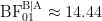
The previous post gave a demonstration of Bayes factor coherence. Specifically, the post considered a test for a binomial parameter \theta, pitting the null hypothesis \mathcal{H}_{0} : \theta = \frac{1}{2} against the alternative hypothesis \mathcal{H}_1: \theta \sim \text{beta}(1,1) (i.e., the uniform distribution from 0 to 1). For fictitious data composed of 5 successes and 5 failures, the Bayes factor equals about 2.71 in favor of \mathcal{H}_0. We then split the data into two batches, batch A featuring only the successes and batch B featuring only the failures. The rules of probability stipulate that the “batch-by-batch” Bayes factor is identical to the “all-data-at-once” Bayes factor. And indeed, \text{BF}_{01}^\text{A} \approx 1/5.33, \text{BF}_{01}^{\text{B}\mid\text{A}} \approx 14.44, such that \text{BF}_{01}^\text{A} \times \text{BF}_{01}^{\text{B}\mid\text{A}} \approx 2.71, as required. This is coherent, and the previous blog post argued that this coherence is due to the fact that the Bayes factor is sensitive to the prior distribution, as the prior encodes the knowledge from the past to generate predictions about the future.

The Bayes Factor Coherence Plot

Bayes factor detractors may argue that batches A and B were cherry-picked, and that this particular sequence of successes and failures is relatively unlikely under the models considered. This objection is both correct and irrelevant. The pattern of coherence is entirely general. To appreciate this, we first write the Bayes factor on a batch-by-batch basis, using the law of conditional probability:

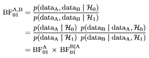
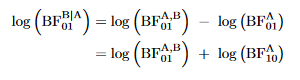
Thus, the coherence of the Bayes factor does not depend on how the batches are constructed. It is insightful to take the logarithm of the Bayes factor and obtain:

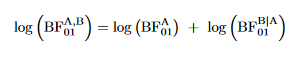
The log transformation accomplishes the following:

  • Multiplication is changed to addition, which is a simpler operation.
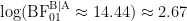
  • Evidence is symmetrized. For regular Bayes factors, positive evidence ranges from 1 to infinity, whereas negative evidence is compressed to the interval from 0 to 1. For instance, \text{BF}_{01} = 20 is of the same evidential strength as \text{BF}_{01} = \frac{1}{20} = 0.05, only differing in direction. This is brought out more clearly when the logarithm is used, as \log(20) \approx 3 and \log(\frac{1}{20}) \approx -3.
  • Evidence in favor of \mathcal{H}_0 (i.e., \text{BF}_{01} > 1) yields a positive number (i.e., \log(\text{BF}_{01}) > 0) whereas evidence in favor of \mathcal{H}_1 (i.e., \text{BF}_{01} < 1) yields a negative number (i.e., \log(\text{BF}_{01}) < 0), with \log(\text{BF}_{01}) = 0 indicating evidential irrelevance or evidential neutrality.

Applying the log transform to our example data yields the result visualized in the figure below, which may be termed a “Bayes factor coherence plot”:

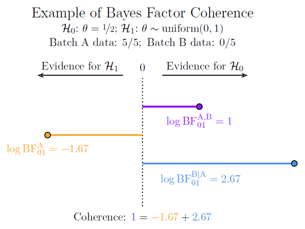
Let’s unpack. The purple line on top indicates the logarithm of the Bayes factor for the complete data set, that is, \log (\text{BF}_{01}^{\text{A,B}} \approx 2.71 ) \approx 1 . The orange line in the middle indicates the logarithm of the Bayes factor for the batch A data, that is, \log (\text{BF}_{01}^{\text{A}} \approx \frac{1}{5.33}) \approx -1.67. Note that the Bayes factor \text{BF}_{01}^{\text{A}} is smaller than 1 (because the batch A data are more likely under \mathcal{H}_1 than under \mathcal{H}_0), which means that the logarithm is negative – the orange line therefore extends to the left rather than the right. The blue line on the bottom indicates the logarithm of the Bayes factor for the batch B data, that is, \log (\text{BF}_{01}^{\text{B} | \text{A}} \approx 14.44) \approx 2.67.

A Bayesian Boomerang

Expressed in the usual way, coherence takes a multiplicative form: 2.71 = \frac{1}{5.33} \times 14.44. After the log transform, coherence is expressed through addition: 1 = -1.67 + 2.67. In our example, the complete data set yielded evidence in favor of \mathcal{H}_0, whereas the data from batch A yielded evidence against \mathcal{H}_0. The Bayes factor coherence plot clarifies that whenever this pattern arises, the batch B data have to provide a log Bayes factor that equals the sum of the log Bayes factor for the complete data and the log Bayes factor for the batch A data. From the earlier equation we have that

Whenever \log (\text{BF}_{01}^{\text{A,B}}) > 0 (i.e., the complete data favor \mathcal{H}_0) and \log (\text{BF}_{10}^{\text{A}}) > 0 (i.e., the batch A data favor \mathcal{H}_1 – mind the Bayes factor subscripts here) we have a “Bayesian evidentiary boomerang”: the batch A data may favor \mathcal{H}_1, but the posterior distribution after batch A yields poor predictions for the data from batch B; the batch A data are not representative of the whole and they have wrong-footed \mathcal{H}_1. The more \mathcal{H}_1 outpredicts \mathcal{H}_0 for the batch A data, the worse it will do for the batch B data (given that the complete data set favors \mathcal{H}_0): inevitably, the evidence trajectory reverses its course and ends up at exactly the same location that is occupied by the “all-data-at-once” Bayes factor.

We may entertain a different division of the data into batches A and B, or we may specify more than two batches – we may even specify each batch to contain a single observation. However the data are subdivided, the end result is always coherent in the sense displayed in the coherence plot: the log Bayes factors for the individual batches are simply added and always yield a result identical to the log Bayes factor for the complete data set.

The main point of this series of blog posts is not to argue that Bayes factors are coherent (even though they are); it is also not to suggest that such coherence is elegant (even though I believe it is); rather, the main point is to demonstrate that the coherence comes about because the Bayes factors are sensitive to the prior distribution. This is a perfect, Goldilocks kind of sensitivity: not too little, not too much, but exactly the right amount in order to ensure that the method does not fall prey to internal contradictions.