A Primer on Bayesian Model-Averaged Meta-Analysis

May 07 - 2020

This post is an extended synopsis of a preprint that is available on PsyArXiv: https://psyarxiv.com/97qup/

Abstract

Meta-analysis is the predominant approach for quantitatively synthesizing a set of studies. If the studies themselves are of high quality, meta-analysis can provide valuable insights into the current scientific state of knowledge about a particular phenomenon. In psychological science, the most common approach is to conduct frequentist meta-analysis. In this primer, we discuss an alternative method, Bayesian model-averaged meta-analysis. This procedure combines the results of four Bayesian meta-analysis models: (1) fixed-effect null hypothesis, (2) fixed-effect alternative hypothesis, (3) random-effects null hypothesis, and (4) random-effects alternative hypothesis. These models are combined according to their plausibilities in light of the observed data to address the two key questions “Is the overall effect non-zero?” and “Is there between-study variability in effect size?”. Bayesian model-averaged meta-analysis therefore avoids the need to select either a fixed-effect or random-effects model and instead takes into account model uncertainty in a principled manner.

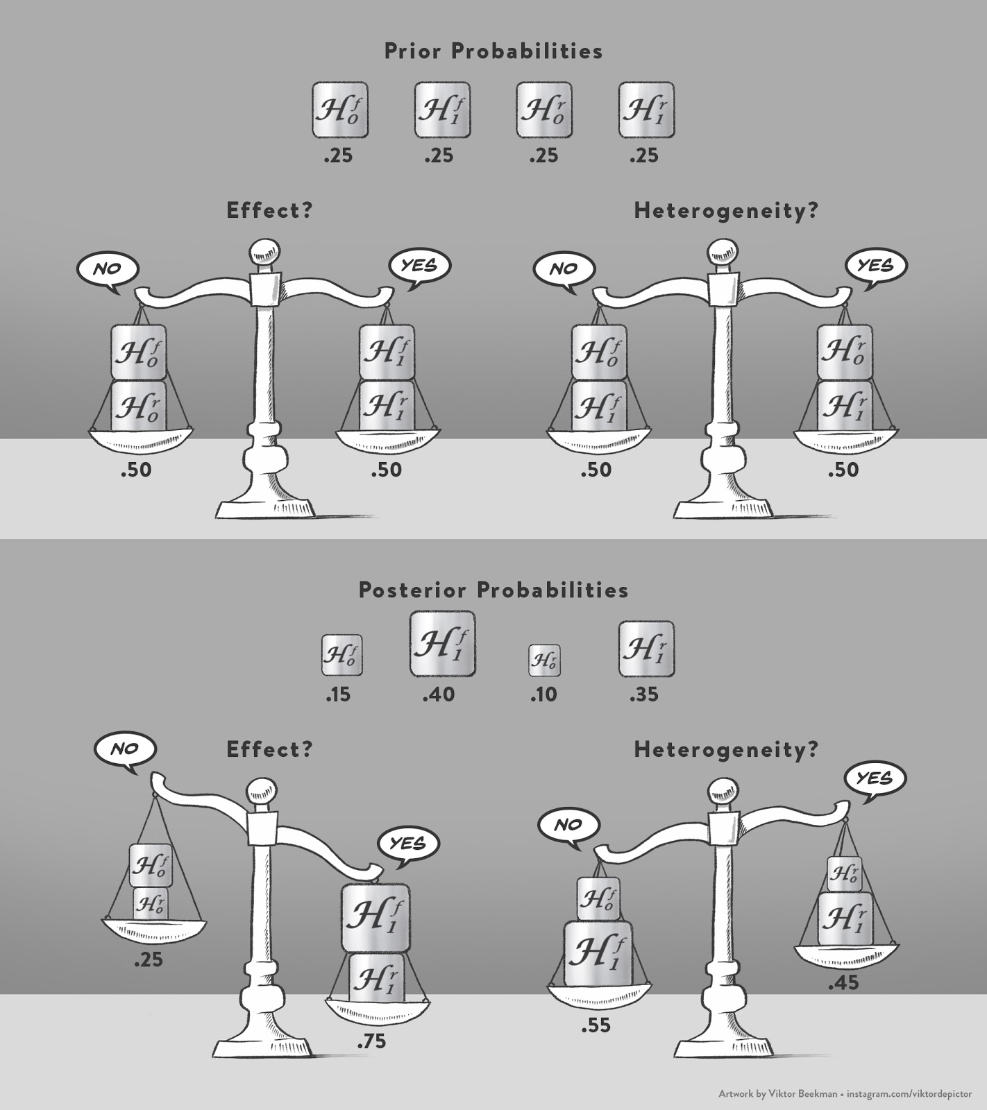
Figure 1. Prior probabilities of the hypotheses and computation of the model-averaged prior inclusion odds (top panel), and exemplary posterior probabilities and computation of the model-averaged posterior inclusion odds (bottom panel). Available at https://www.bayesianspectacles.org/library/ under CC license https://creativecommons.org/licenses/by/2.0/.

Example: Testing the Self-Concept Maintenance Theory

According to the self-concept maintenance theory (Mazar et al., 2008), people will cheat to maximize self-profit, but only to the extent that they can still maintain a positive self-view. In their Experiment 1, Mazar et al. gave participants an incentive and opportunity to cheat. Before working on a problem-solving task, participants either recalled, as a moral reminder, the Ten Commandments, or, as a neutral condition, they recalled 10 books they had read in high school. In line with the self-concept maintenance hypothesis, participants in the moral reminder condition reported having solved fewer problems than those in the neutral condition which also reflected their actual performance better. Recently, a Registered Replication Report (Verschuere et al., 2018) attempted to replicate this finding. Here we focus on the primary meta-analysis that included data from 19 labs.

Parameter Prior Settings

We use three different parameter prior specifications. These specifications differ only in the prior for the effect size $\mu$ as the prior for the between-study standard deviation $\tau$ is always an Inverse-Gamma(1, 0.15) distribution. The first specification assigns $\mu$ a default zero-centered Cauchy prior distribution with scale $1/\sqrt{2}$ . This specification will be referred to as Default (Two-Sided). The second specification is very similar, but truncates the default Cauchy prior distribution at zero in order to incorporate the directedness of the self-concept maintenance hypothesis (i.e., participants in the Ten Commandments condition are expected to cheat less than participants in the neutral condition, not more). This specification will be referred to as Default (One-Sided). Finally, the third specification uses as an informed prior for $\mu$ a $t$ distribution that is centered on -0.35, with scale 0.102 and three degrees of freedom. This prior is also truncated at zero to preclude effect sizes in the direction opposite to what the hypothesis predicts. This “Oosterwijk” prior has been elicited for a reanalysis of a social psychology study (Gronau et al., in press), but we believe it is a reasonable prior for psychological studies more generally.¹ This specification will be referred to as Informed (One-Sided).

Hypotheses Posterior Probabilities

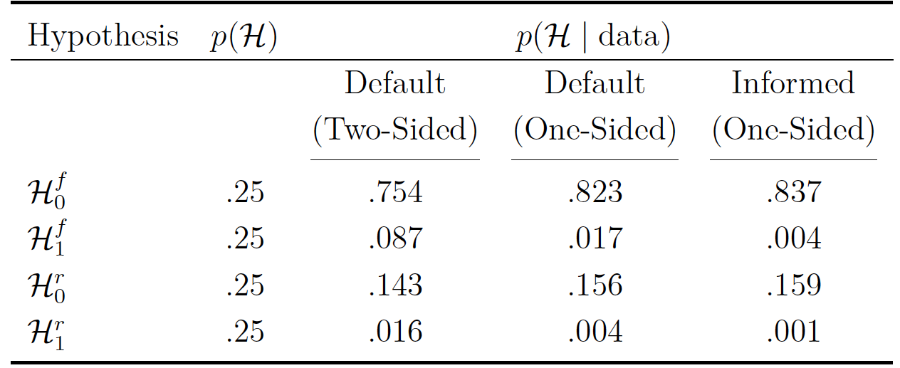
Table 1. Prior and posterior probabilities of the four hypotheses of interest for the Verschuere et al. (2018) Registered Replication Report data. The posterior probabilities are displayed for three different prior settings for the effect size parameter $\mu$ .

Model-Averaged Bayes Factor for an Overall Effect

To address the question whether the meta-analytic effect is non-zero (i.e., Q1), we compute the model-averaged Bayes factor $\text{BF}_{10}$ for each prior setting. This can be achieved solely based on the probabilities presented in Table 1. For the Default (Two-Sided) prior setting, the posterior inclusion odds for an effect are given by $(.087 + .016) / (.754 + .143) \approx 0.115$ . Since the prior inclusion odds are equal to one, this number equals the model-averaged Bayes factor, $\text{BF}_{10} \approx 0.115$ . Consequently, $\text{BF}_{01} = 1/\text{BF}_{10} \approx 8.696$ indicating moderate evidence for the absence of an effect.
For the Default (One-Sided) prior setting, the posterior inclusion odds for an effect are given by $(.017 + .004) / (.823 + .156) \approx 0.021$ ; this number equals the model-averaged Bayes factor, $\text{BF}_{10} \approx 0.021$ . Consequently, $\text{BF}_{01} = 1/\text{BF}_{10} \approx 47.619$ indicating very strong evidence for the absence of an effect.
For the Informed (One-Sided) prior setting, the posterior inclusion odds are calculated in the same fashion. The model-averaged Bayes factor is therefore $\text{BF}_{10} \approx (.004 + .001) / (.837 + .159) \approx 0.005$ . Consequently, $\text{BF}_{01} = 1/\text{BF}_{10} \approx 200$ indicating extreme evidence for the absence of an effect. In sum, for all prior settings, the model-averaged Bayes factor indicates evidence in favor of the null hypothesis of no effect. However, the degree of evidence differs across prior settings. The reason why the Default (One-Sided) and the Informed (One-Sided) prior setting yield more evidence for the absence of an effect is that, as reported by Verschuere et al., the meta-analytic effect goes in the direction opposite of what the theory predicts and these priors for $\mu$ do not assign any mass to population effect size values that go in the opposite direction.

Sequential Analysis

For this particular example, studies were conducted at about the same time and we do not know the order in which they finished. However, in other cases the temporal order may be known and of interest. This is especially the case for meta-analyses combining studies from several decades where trends in the field may affect study design and results. Here we demonstrate how to conduct a sequential analysis that displays the evidence as studies accumulate. Since the presented approach is Bayesian, current knowledge can be updated by new evidence without having to worry about optional stopping (Rouder, 2014). To demonstrate the sequential analysis, we make the arbitrary assumption that the temporal order of the studies coincides with the alphabetical order of the last names of the labs’ leading researchers. Furthermore, for demonstration purposes, we focus on one prior setting, Default (Two-Sided). Figure 2 displays how the posterior probability for each of the four hypotheses changes as studies accumulate.

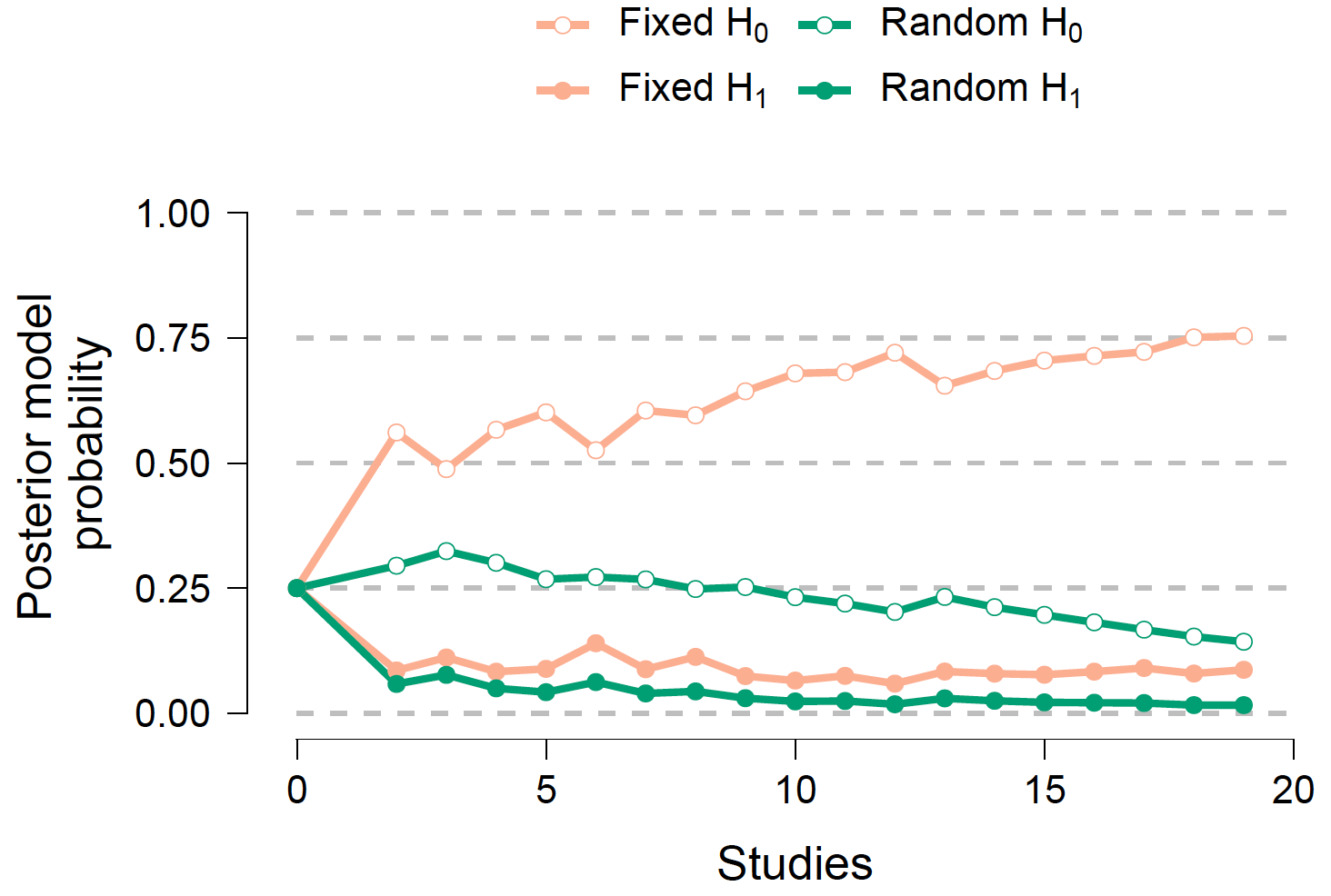
Figure 2. Sequential analysis. The posterior probability for each of the four hypotheses
is displayed as a function of the number of studies included in the analysis. Figure
from JASP (jasp-stats.org/).

Concluding Comments

Bayesian model-averaged meta-analysis affords researchers the well-known pragmatic benefits of a Bayesian method. In addition, it allows researchers to take into account model uncertainty with respect to choosing a fixed-effect or random-effects model when addressing the two key questions “Is the overall effect non-zero?”’ (Q1) and “Is there between-study variability in effect size?” (Q2).

Notes

¹ We flipped the sign of the location parameter to align with the way the data are coded (i.e., the theory predicts negative effect sizes).

References

Gronau, Q. F., Heck, D. W., Berkhout, S. W., Haaf, J. M., & Wagenmakers, E.-J. (2020). A primer on Bayesian model-averaged meta-analysis. Manuscript submitted for publication. https://psyarxiv.com/97qup/

Gronau, Q. F., Ly, A., & Wagenmakers, E.-J. (in press). Informed Bayesian t-tests. The
American Statistician. Retrieved from https://arxiv.org/abs/1704.02479

Mazar, N., Amir, O., & Ariely, D. (2008). The dishonesty of honest people: A theory of
self-concept maintenance. Journal of Marketing Research, 45, 633-644.

Rouder, J. N. (2014). Optional stopping: No problem for Bayesians. Psychonomic Bulletin & Review, 21, 301-308.

Verschuere, B., Meijer, E. H., Jim, A., Hoogesteyn, K., Orthey, R., McCarthy, R. J., . . .Yıldız, E. (2018). Registered Replication Report on Mazar, Amir, and Ariely (2008). Advances in Methods and Practices in Psychological Science, 1, 299-317.

About The Authors

Quentin F. Gronau

Quentin is a PhD candidate at the Psychological Methods Group of the University of Amsterdam.

Daniel Heck

Daniel Heck is professor of Psychological Methods at the Philipps University of Marburg, Germany.

Sophie Berkhout

Sophie Berkhout is a Research Master student in Psychology at the University of Amsterdam.

Julia Haaf

Julia Haaf is postdoc at the Psychological Methods Group at the University of Amsterdam.

Eric-Jan Wagenmakers

Eric-Jan (EJ) Wagenmakers is professor at the Psychological Methods Group at the University of Amsterdam.

Blog