The Single Most Prevalent Misinterpretation of Bayes’ Rule

December 20 - 2018

We thank Alexander Ly for constructive comments on an earlier draft of this post.

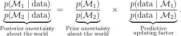
Bayes’ rule tells us how to learn from experience, that is, by updating our knowledge about the world using relative predictive performance: hypotheses that predicted the data relatively well receive a boost in credibility, whereas hypotheses that predicted the data relatively poorly suffer a decline (e.g., Wagenmakers et al., 2016). This predictive updating principle holds for propositions, hypotheses, models, and parameters: every time, our uncertainty is updated using the same mathematical operation. Take for instance the learning process involving just two models, $\mathcal{M}$ ₁ and $\mathcal{M}$ ₂ (but note that these may equally well refer to parameter values, say $\theta$ ₁ and $\theta$ ₂, within a single model). The odds form of Bayes’ rule yields

$\underbrace{ \frac{p(\mathcal{M}_1 \mid \text{data})}{p(\mathcal{M}_2 \mid \text{data})}}_{\substack{\text{Posterior uncertainty}\\ \text{about the world}} } = \underbrace{ \frac{p(\mathcal{M}_1)}{p(\mathcal{M}_2)}}_{\substack{\text{Prior uncertainty}\\ \text{about the world}} } \times \,\,\,\,\,\,\, \underbrace{ \frac{p(\text{data} \mid \mathcal{M}_1)}{p(\text{data} \mid \mathcal{M}_2)}}_{\substack{\text{Predictive}\\ \text{updating factor} } }.$

This equation shows that the change from prior odds to posterior odds is brought about by a predictive updating factor that, for model selection, is widely known as the Bayes factor (e.g., Etz & Wagenmakers, 2017) So we have prior knowledge, we use it to make predictions, and the adequacy of these predictions drives an optimal, cyclical learning process that is visualized in the figure below:

Bayesian learning can be conceptualized as a cyclical process of updating knowledge in response to prediction errors. The prediction step is deductive, and the updating step is inductive. For a detailed account see Chapters XI and XII in Jevons (1874/1913).

Intuitive and elegant, the Bayesian formalism does not seem to leave much room for grotesque misinterpretation concerning, for instance, hypothetical data sets with imaginary results that depend on intentions accessible only to the experimenter at the time of data collection (e.g., Berger & Wolpert, 1988). We present the algorithm again, in words:

$\substack{\text{\normalsize{Present uncertainty}}\\ \text{\normalsize{about the world}}} \, = \, \substack{\text{\normalsize{Past uncertainty}}\\ \text{\normalsize{about the world}}} \,\,\, \times \,\, \substack{\text{\normalsize{Predictive}}\\ \text{\normalsize{updating factor}}}$

The most common misinterpretation is to confuse the predictive updating factor, that is, the evidence, with the end result — the present uncertainty. If $\mathcal{M}$ ₁ predicted the data five times better than $\mathcal{M}$ ₂, this emphatically does not mean that $\mathcal{M}$ ₁ is now five times more plausible than $\mathcal{M}$ ₂. That interpretation is valid only when the two models were equally plausible a priori (i.e., the prior odds are 1). This may seem like an inconsequential mistake to make, but it is fundamental. What the predictive updating factor or Bayes factor tells us is the degree to which the data should shift our opinion; it is the evidence that is provided by the data. But our final opinion may be very different from the evidence. A few brief examples follow:

Example 1: The Data Provide No Evidence At All

Billy Bob, a history undergrad, needs to write a report on whether the 1969 Apollo 11 moon landing was real news ( $\mathcal{M}$ ₁; a hypothesis that Billy Bob deems highly plausible a priori) or fake news ( $\mathcal{M}$ ₂; a hypothesis that Billy Bob deems highly implausible a priori). Instead of preparing in earnest, Billy Bob spends all his time playing Mario Kart 8 Deluxe with his friends. Billy Bob’s Mario Kart scores are equally likely under $\mathcal{M}$ ₁ and $\mathcal{M}$ ₂, and hence the predictive updating factor is 1: we have not learned anything and the data can be said to be predictively irrelevant. But it would be a grave and obvious mistake to conclude from Billy Bob’s scores that we have learned that, since the Bayes factor is 1, $\mathcal{M}$ ₁ and $\mathcal{M}$ ₂ are now equally plausible. The next example features data that are predictively relevant.

Example 2: Extrasensory Perception

In 2011, Daryl Bem published an infamous article in which he argued that people have precognition, a form of extrasensory perception that allows them to predict the future (Bem, 2011). In Bem’s first experiment, “Precognitive Detection of Erotic Stimuli”, each of 100 Cornell undergraduates were asked to guess, repeatedly, which of two curtains on the computer screen was hiding a picture. As the location of the picture was determined randomly, participants could perform reliably better than chance (50%) only if they had precognition. The results were as follows:

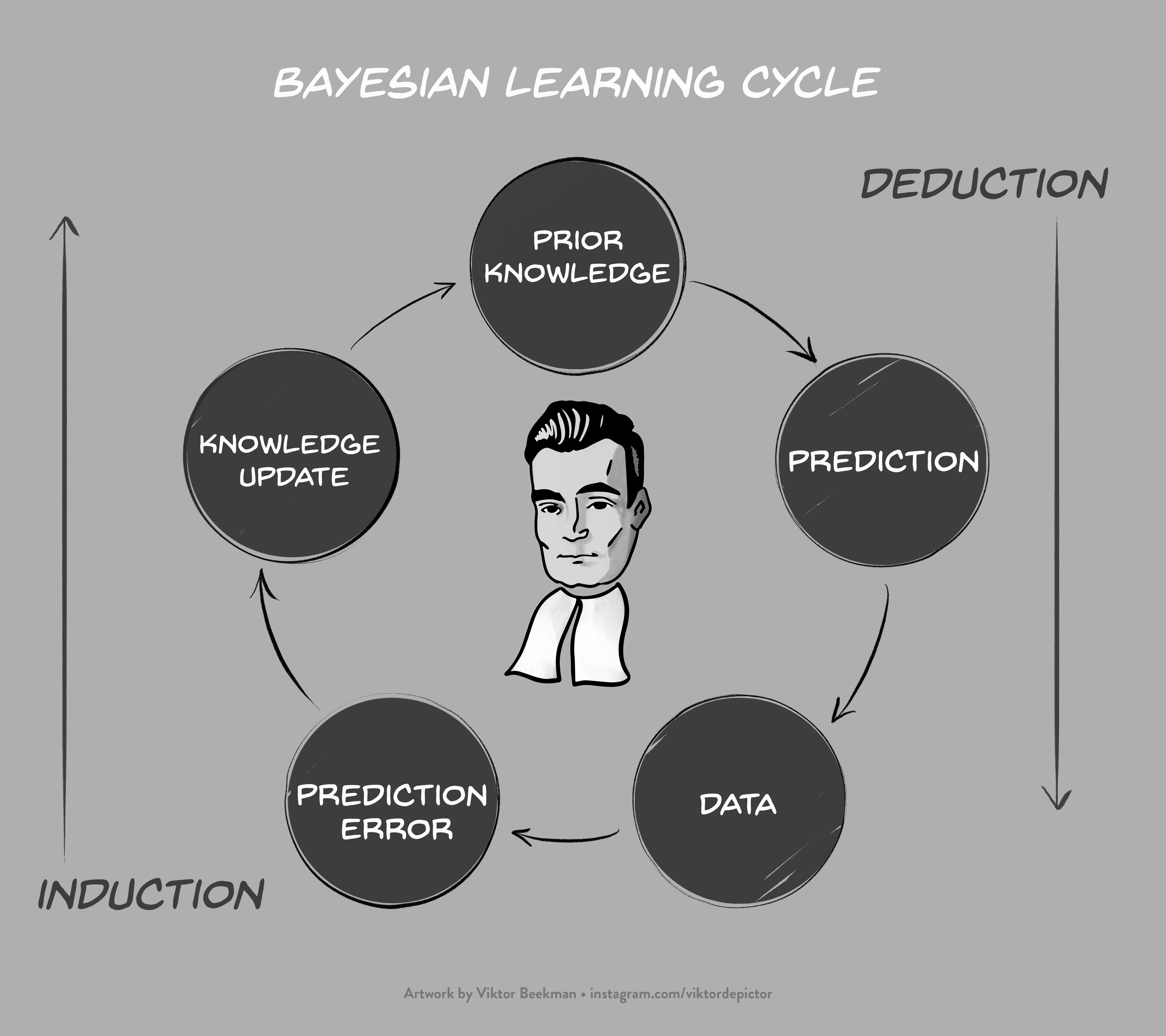
“Across all 100 sessions, participants correctly identified the future position of the erotic pictures significantly more frequently than the 50% hit rate expected by chance: 53.1%, t(99) = 2.51, p = .01, d = 0.25.” (Bem, 2011, p. 409)

We can analyze these data in JASP (jasp-stats.org) using the Summary Stats module (Ly et al., in press). We select the “one sample t-test”, add “2.51” for the t-value and “100” for the group size. The result is a Bayes factor of about 2 in favor of the precognition hypothesis over the null hypothesis, a level of evidence that is relatively weak.

JASP screenshot of the default Bayesian test for the results of Daryl Bem’s 2011 Experiment 1, “Precognitive Detection of Erotic Stimuli”. With a Bayes factor of 2.168, the evidence for precognition is relatively weak.

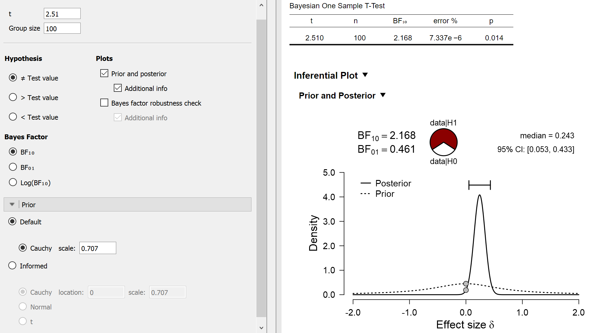
However, we can try different analyses by changing our expectations for effect size under the precognition hypothesis. For instance, we may include an order-restriction and only predict positive effects, that is, precognition only acts to increase, not decrease, detection rates. We might also use a more informed distribution (Gronau et al., 2018); for illustrative purposes we will use the “Oosterwijk prior”, a generic prior for small to medium effects. The Oosterwijk prior is a t-distribution with location 0.350, scale 0.102, and 3 degrees of freedom. The results of the informed analysis are shown below:

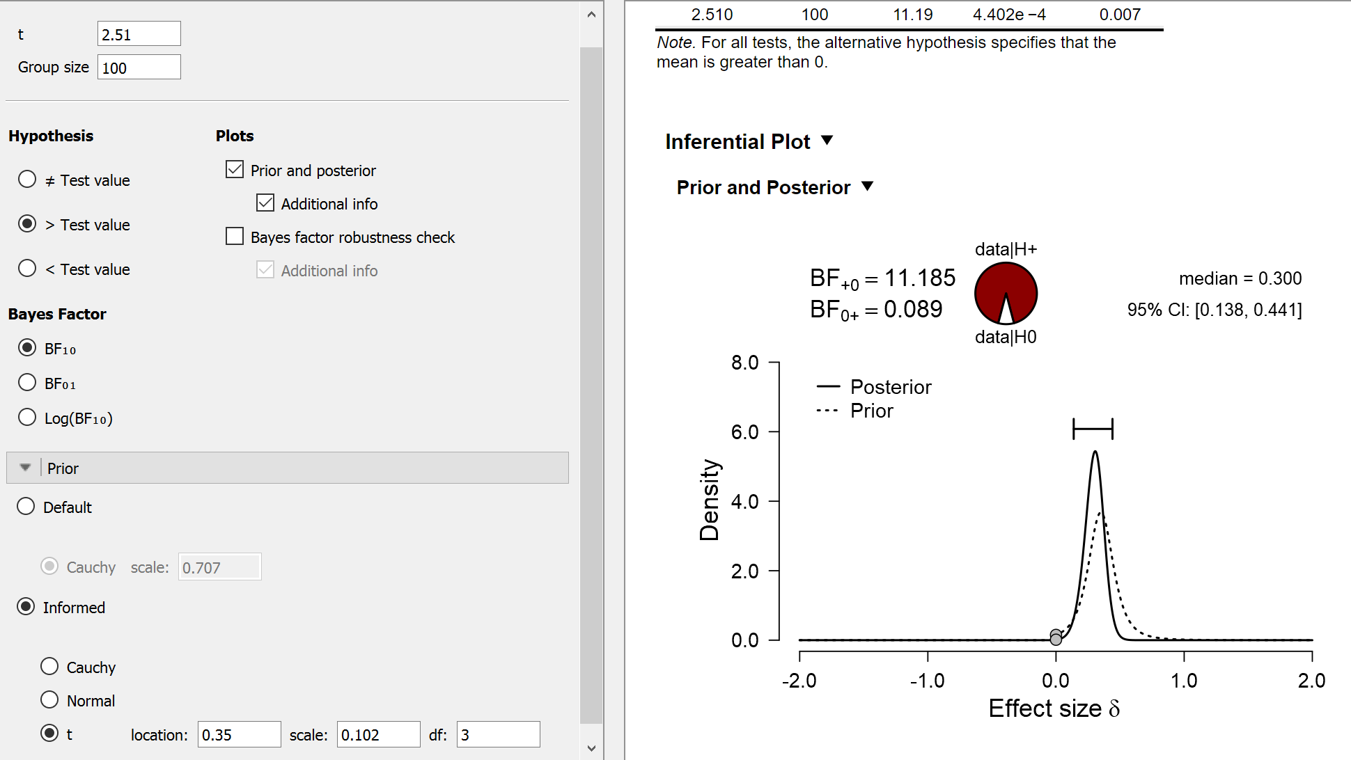
JASP screenshot of the default Bayesian test for the results of Daryl Bem’s 2011 Experiment 1, “Precognitive Detection of Erotic Stimuli”. With a Bayes factor of 11.185, the evidence for precognition is clearly stronger than it was before.

The new analysis shows that the Bayes factor equals about 11. Now there are some serious issues with these data and with this particular analysis, but for the moment we will let that slide and just consider the Bayes factor of 11 in favor of precognition. Does this result (taken at face value) mean that the precognition hypothesis is now 11 times more plausible than the skeptics’ null hypothesis? Of course not: the precognition hypothesis is highly unlikely a priori, and the Bayes factor only looks at the change in beliefs that is brought about by the data. Thus, even though your change in belief brought about by the data might be considerable, your beliefs about the world may not have changed much in absolute terms. A very, very small number multiplied with a very large number still yields a very small number, see the first equation above. The next example illustrates this on a classic textbook example.

Example 3: Drunk Driving and the Base Rate Fallacy

The prototypical demonstration of the fact that evidence does not equal posterior belief is given by the base rate fallacy: a test with fantastic operating characteristics may actually provide a deeply misleading impression of the final belief state. The basic problem features in every textbook on probability, and it is usually concluded that the Bayesian solution is too complicated for people to wrap their heads around. Indeed, the Bayesian solution is complicated when it is presented as a single step. Break it down into its component steps, and the process becomes much simpler.

Let’s consider the same problem as is mentioned on the Wikipedia page for the base rate fallacy:

“A group of police officers have breathalyzers displaying false drunkenness in 5% of the cases in which the driver is sober. However, the breathalyzers never fail to detect a truly drunk person. One in a thousand drivers is driving drunk. Suppose the police officers then stop a driver at random, and force the driver to take a breathalyzer test. It indicates that the driver is drunk. We assume you don’t know anything else about him or her. How high is the probability he or she really is drunk? Many would answer as high as 95%, but the correct probability is about 2%.”

In the first step of our Bayesian analysis of this problem, we take stock of our prior information: “one in a thousand drivers is driving drunk”. This means that p(drunk) = $\frac{1}{1000}$ and p(sober) = $\frac{999}{1000}$ . So, before we see any data, the prior odds in favor of someone being sober instead of drunk are

$\frac{p(\text{sober})}{p(\text{drunk})} = 999$ .

In the second step we consider the evidence that is provided by the data. We know that the breathalyzer test is positive. The probability of this happening for drunk drivers is 1, and for sober drivers it is .05. The Bayes factor in favor of the driver being drunk rather than sober is therefore: p(test positive | drunk) / p(test positive | sober) = 1/.05 = 20.

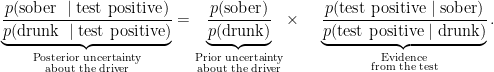
In the third step we combine our prior information (i.e., odds of 999 in favor of the driver being sober) with the evidence from the test (i.e., a Bayes factor of 20 in favor of the driver being drunk) in order to arrive at the posterior odds, that is, p(drunk | test positive) / p(sober | test positive). The odds for the driver being sober were 999 prior to the test result; the test result, however, is positive and this requires a downward adjustment by a factor of 20, so that the posterior odds for the driver being sober have been reduced to 999/20 = 49.95. This step is intuitive but can be formalized by rewriting our first equation as follows:

$\underbrace{ \frac{p(\text{sober } \mid \text{test positive})}{p(\text{drunk } \mid \text{test positive})}}_{\substack{\text{Posterior uncertainty}\\ \text{about the driver}} } = \underbrace{ \frac{p(\text{sober})}{p(\text{drunk})}}_{\substack{\text{Prior uncertainty}\\ \text{about the driver}} } \times \,\,\,\,\,\,\, \underbrace{ \frac{p(\text{test positive} \mid \text{sober})}{p(\text{test positive} \mid \text{drunk})}}_{\substack{\text{Evidence}\\ \text{from the test} } }.$

In the final step, we transform the posterior odds of 49.95 for the driver being sober to a posterior probability: p(sober | test positive) = 49.95 / (49.95+1) $\approx$ 0.98. This means that even after a positive breathalyzer test outcome, the probability that a given driver is drunk is still only about 2%.

The standard Bayesian solution to the base rate fallacy involves the law of total probability in order to compute p(positive test) as p(positive test | drunk)p(drunk) + p(positive test | sober)p(sober) and then use this as the denominator in a fraction with p(positive test | drunk)p(drunk) as the numerator. The end-result is obtained in one step, but requires three simultaneous operations: multiplication, addition, and division. In contrast, the odds form of Bayes’ rule is intuitive and immediately clarifies the importance of the prior odds and the separate role of evidence.¹

Example 4: Popper on Corroboration

Karl Popper was notoriously grumpy (and deeply mistaken, in our opinion²) about all things Bayesian. One example is relevant for our current discussion. Here Popper (1959) wishes to demonstrate that degree of corroboration cannot be identified with a probability³:

“Consider the next throw with a homogeneous die. Let $x$ be the statement ‘six will turn up’; let $y$ be its negation, that is to say, let $y=\bar{x}$ ; and let $z$ be the information ‘an even number will turn up’.

We have the following absolute probabilities:

$p(x) = 1/6; \quad p(y) = 5/6; \quad p(z) = 1/2.$

Moreover, we have the following relative probabilities:

$p(x|z) = 1/3; \quad p(y|z) = 2/3.$

We see that $x$ is supported by the information $z$ , for $z$ raises the probability of $x$ from $1/6$ to $2/6 = 1/3$ . We also see that $y$ is undermined by $z$ , for $z$ lowers the probability of $y$ by the same amount from $5/6$ to $4/6 = 2/3$ . Nevertheless, we have p(x|z) < p(y|z).
[…] expresses a fact we have established by our example: that $x$ may be supported by $z$ , and $y$ undermined by $z$ , and that nevertheless $x$ , given $z$ , may be less probable than $y$ , given $z$ .
[…] Thus we have proved that the identification of degree of corroboration or confirmation with probability is absurd on both formal and intuitive grounds: it leads to self-contradiction.” (Popper, 1959, pp. 390-391)

Popper’s demonstration is yet another example of the fact that evidence does not equal posterior belief. We started with prior odds p(y)/p(x) = 5, favoring $y$ over $x$ by a factor of 5. Then we obtained knowledge that $z$ holds — an even number has turned up. The probability of this happening under $x$ (‘six will turn up’) is 1, whereas under $y$ (‘either 1, 2, 3, 4, or 5 will turn up, with equal probability’) that probability is 2/5. Consequently, the knowledge that $z$ holds is associated with an updating factor that favors $x$ over $y$ , and by p(z|x)/p(z|y) = 5/2. This updating factor –a ratio, indeed not a probability– is the degree of corroboration that the information $z$ provides for the rival hypotheses $x$ and $y$ . Multiplying the prior odds with the updating factor yields a posterior odds that still favors $y$ over $x$ , albeit by a lesser amount than before, as 5 $\times \frac{2}{5}$ = 2.

To conclude, in Popper’s example the statement $y$ was five times more likely a priori than the statement $x$ . Information $z$ provided some evidence for $x$ over $y$ , but after this is taken into account $y$ is still twice as likely as $x$ . The structure of this problem is the same as that of the base rate fallacy.

We hope that these four examples helped clarify a misinterpretation of Bayes’ rule that is common among newcomers to Bayesian inference: change in belief does not equal posterior belief.

Footnotes

¹ For a more extensive treatment see one of John Kruschke’s blog posts.

² An opinion we are honored to share with Harold Jeffreys.

³ In the fragment below we have modernized Popper’s notation for conditional probability.

References

Bem, D. J. (2011). Feeling the future: Experimental evidence for anomalous retroactive influences on cognition and affect. Journal of Personality and Social Psychology, 100, 407-425.

Berger, J. O., & Wolpert, R. L. (1988). The Likelihood Principle (2nd ed.). Hayward (CA): Institute of Mathematical Statistics.

Gronau, Q. F., Ly, A., & Wagenmakers, E.-J. (2018). Informed Bayesian t-tests. Manuscript submitted for publication. Available at https://arxiv.org/abs/1704.02479.

Ly, A., Raj, A., Marsman, M., Etz, A., & Wagenmakers, E.-J. (2018). Bayesian Reanalyses from summary statistics: A guide for academic consumers. Advances in Methods and Practices in Psychological Science, 3, 367-374. Open Access.

Popper, K. R. (1959). The Logic of Scientific Discovery. New York: Harper Torchbooks.

Wagenmakers, E.-J., Morey, R. D., & Lee, M. D. (2016). Bayesian benefits for the pragmatic researcher. Current Directions in Psychological Science, 25, 169-176.

About The Authors

Eric-Jan Wagenmakers

Eric-Jan (EJ) Wagenmakers is professor at the Psychological Methods Group at the University of Amsterdam.

Alexander Etz

Alexander is a PhD student in the department of cognitive sciences at the University of California, Irvine.

Quentin Gronau

Quentin is a PhD candidate at the Psychological Methods Group of the University of Amsterdam.

Fabian Dablander

Fabian is a PhD candidate at the Psychological Methods Group of the University of Amsterdam. You can find him on Twitter @fdabl.

Blog

The Single Most Prevalent Misinterpretation of Bayes’ Rule

Search

Categories

follow us