Preprint: doi:10.31234/osf.io/wgb64

Abstract

“Many statistical scenarios initially involve several candidate models that describe the data-generating process. Analysis often proceeds by first selecting the best model according to some criterion, and then learning about the parameters of this selected model. Crucially however, in this approach the parameter estimates are conditioned on the selected model, and any uncertainty about the model selection process is ignored. An alternative is to learn the parameters for all candidate models, and then combine the estimates according to the posterior probabilities of the associated models. The result is known as Bayesian model averaging (BMA). BMA has several important advantages over all-or-none selection methods, but has been used only sparingly in the social sciences. In this conceptual introduction we explain the principles of BMA, describe its advantages over all-or-none model selection, and showcase its utility for three examples: ANCOVA, meta-analysis, and network analysis.”

The Railway Station

“Imagine waiting at a railway station for a train that is supposed to take you to an important meeting. The train is running a few minutes late, and you start to deliberate whether or not to use an alternative mode of transportation. In your deliberation, you contemplate the different scenarios that could have transpired to cause the delay. There may have been a serious accident, which means your train will be delayed by several hours. Or perhaps your train has been delayed by a hail storm and is likely to arrive in the next half hour or so. Alternatively, your train could have been stuck behind a slightly slower freight train, which means that it could arrive at any moment. In your mind, each scenario i corresponds to a model of the world Hi that is associated with a different distribution of estimated delay t, denoted p(t | Hi). You do not know the true scenario H’, but you don’t really care about it either; in your hurry, all that is relevant for your decision to continue waiting or to take action is the expected delay p(t) unconditional on any particular model Hi.”

Bayesian Model Averaging

“In probabilistic terms, we call p(t) the Bayesian model averaging (BMA) estimate. Rather than first selecting the single most plausible scenario H and then using p(t | H) for all decisions and conclusions, BMA provides an assessment of the delay t that takes into account all scenarios simultaneously. This is accomplished by computing a weighted average, where the weights quantify the plausibility of each scenario. For instance, while it is in principle possible that the railway company has decided to start major construction work today, thus causing a delay of weeks, most likely you would have learned about this sooner. Therefore, the prior model plausibility Hi of this scenario is low, and its implied long delay contributes only little to p(t).”

Pandemonium

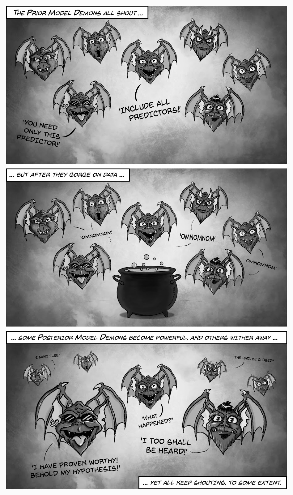
“The intuition for BMA can be illustrated by the `Bayesian model averaging pandemonium’. Here, the different candidate models are represented by a legion of demons, and their sizes reflect their probabilities. Some demons grow when they are presented with observations that are consistent with them, while observations inconsistent with a demon causes it to shrink. If this process fails to identify a single dominant demon, it is prudent to listen to all of them, while weighing their contributions by their sizes, instead of depending entirely on the single best one.”

Examples of Bayesian model averaging

We showcase the application of BMA in a couple of examples, for instance in AnCoVa:

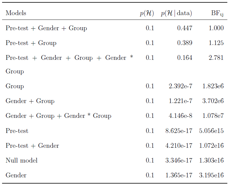
Model comparison for the Bayesian ANCOVA on the Test Anxiety Score data of Shen et al. (2018) featuring the predictors Gender, Group, and Pre-test. The prior model distribution is uniform (i.e., p(Hi)=1/10). The models are sorted by their posterior model probability p(Hi | data). All models are compared to the best model shown in the top row, and hence all Bayes factors, BFtj are larger than one.

The BMA allows us to look at the inclusion probability of each of the considered predictors, which is particularly useful if the number of considered models is too large to tabulate. We find:

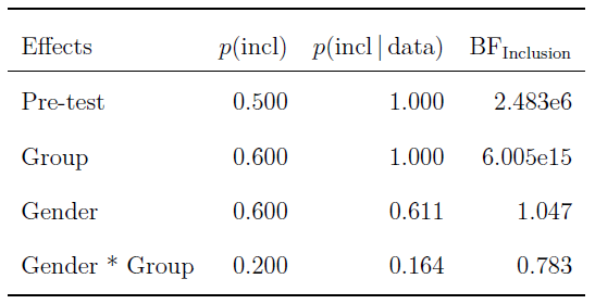
For each predictor, we show its prior inclusion probability (that is, the summed prior probability for the models that feature the predictor), and its posterior inclusion probability. The inclusion Bayes factor indicates how much more likely the observations are under models that include the predictor versus under those that exclude the predictor. The results are sorted by their posterior inclusion probability.

Another example is meta-analysis, where the results of 17 facial feedback studies are combined. Using BMA, we average over the models that contain fixed-effects, random-effects, or no effect at all:

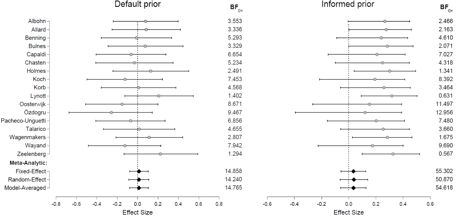
“The estimated effect sizes of the 17 facial feedback studies in the Registered Replication Report (Wagenmakers et al., 2016), for two different prior distributions. Shown are the 95% highest density intervals (horizontal bars) and the median (circles) of the posterior distributions of effect sizes, given δ≠0. In addition, the Bayes factor BF0+ provides the evidence of H0 versus H1, that is, how much more likely the data are under the absence than under the presence of an effect. For instance, the Zeelenberg experiment yields a BF0+ of 1.294 under the default prior, indicating only a smidgen of evidence for the absence of an effect. The bottom three rows indicate the estimated effect size via the meta-analysis models with fixed effect and with random effects, and the BMA of the two. The figure shows that most individual studies provide only weak evidence for the absence of an effect. The meta-analytic BMA averages over both the models with zero effect size and those with nonzero effect size, and is much more compelling.”

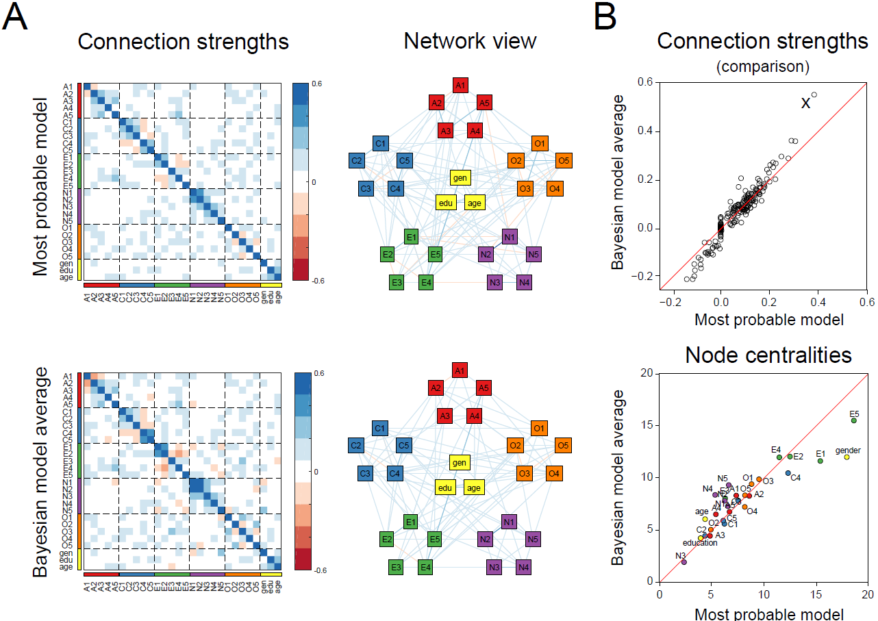
“A comparison of model selection versus model averaging for network analysis on the Big Five personality traits data set. A. The most likely network, as well as the BMA estimate. Shown are both the adjacency matrix and the equivalent network structure. Connection weights represent partial correlations. B. A comparison of the strengths of all connections as well as of betweenness centrality. A number of connections are estimated differently, such as the one indicated with an ‘x’ (representing the connection between traits ‘N1’ (‘getting angry easily’) and ‘N2’ (‘getting irritated easily’)), which has a partial correlation of 0.38 in the selected model, and 0.55 in the BMA estimate. For betweenness centrality, we see traits ‘gender’ as well as ‘E1’ and ‘E5’ are estimated differently.”

Conclusion

BMA is particularly useful when there is uncertainty about the underlying model, while at the same time the model itself is not of primary concern. Consider the example from our introduction again; we are interested in the estimated arrival time of our train, not so much in the particulars of each considered scenario. Just as how we are used to being explicit about the uncertainty of our parameter estimates, for example by making predictions according to the posterior distribution rather than a point estimate, we should also be clear that we are rarely totally confident about which model best accounts for our data. Here too, uncertainty must be taken into account, and BMA provides an elegant way to do so.

References

Hinne, M., Gronau, Q. F., van den Bergh, D., & Wagenmakers, E.-J. (2019). A conceptual introduction to Bayesian model averaging. Manuscript posted on PsyArXiv.

Shen, L., Yang, L., Zhang, J., & Zhang, M. (2018). Benefits of expressive writing in reducing test anxiety: A randomized controlled trial in Chinese samples. PLoS ONE, 13(2), e0191779.

Wagenmakers, E., Beek, T., Dijkhoff, L., & Gronau, Q. F. (2016). Registered Replication Report: Strack, Martin, & Stepper (1988). Association for Psychological Science,11(6), 917–928.

About The Authors

Max Hinne

Max is a post-doctoral researcher at the Department of Psychology at the University of Amsterdam.

Quentin Gronau

Quentin is a PhD candidate at the Psychological Methods Group of the University of Amsterdam.

Don van den Bergh

Don is a PhD candidate at the Department of Psychological Methods at the University of Amsterdam.

Eric-Jan Wagenmakers

Eric-Jan (EJ) Wagenmakers is professor at the Psychological Methods Group at the University of Amsterdam.