This post is an extended synopsis of a preprint that is available on PsyArXiv.
“[…] if you can’t do simple problems, how can you do complicated ones?” — Dennis Lindley (1985, p. 65)
Cross-validation (CV) is increasingly popular as a generic method to adjudicate between mathematical models of cognition and behavior. In order to measure model generalizability, CV quantifies out-of-sample predictive performance, and the CV preference goes to the model that predicted the out-of-sample data best. The advantages of CV include theoretic simplicity and practical feasibility. Despite its prominence, however, the limitations of CV are often underappreciated. We demonstrate with three concrete examples how Bayesian leave-one-out cross-validation (referred to as LOO) can yield conclusions that appear undesirable.
Bayesian Leave-One-Out Cross-Validation
The general principle of cross-validation is to partition a data set into a training set and a test set. The training set is used to fit the model and the test set is used to evaluate the fitted model’s predictive adequacy. LOO repeatedly partitions the data set into a training set which consists of all data points except one and then evaluates the predictive density for the held-out data point where predictions are generated based on the leave-one-out posterior distribution. The log of these predictive density values for all data points is summed to obtain the LOO estimate. LOO can be also used to compute model weights that are on the probability scale and therefore relatively straightforward to interpret.
Example 1: Induction
As a first example, we consider what is perhaps the world’s oldest inference problem, one that has occupied philosophers for over two millennia: given a general law such as “all X’s have property Y”, how does the accumulation of confirmatory instances (i.e., X’s that indeed have property Y) increase our confidence in the general law? Examples of such general laws include “all ravens are black”, “all apples grow on apple trees”, “all neutral atoms have the same number of protons and electrons”, and “all children with Down syndrome have all or part of a third copy of chromosome 21”.
To address this question statistically we can compare two models. The first model corresponds to the general law and can be conceptualized as  , where
  is a Bernoulli rate parameter. This model predicts that only confirmatory instances are encountered. The second model relaxes the general law and is therefore more complex; it assigns a prior distribution, which, for mathematical convenience, we take to be from the beta family — consequently, we have
  . In the following, we assume that, in line with the prediction from
  , only confirmatory instances are observed.
as a function of the number of confirmatory instances  , evaluated in relation to five different prior specifications for
  : (a)
: (a)  ; (b)
; (b)  ; (c)
; (c)  ; (d)
; (d)  ; (e)
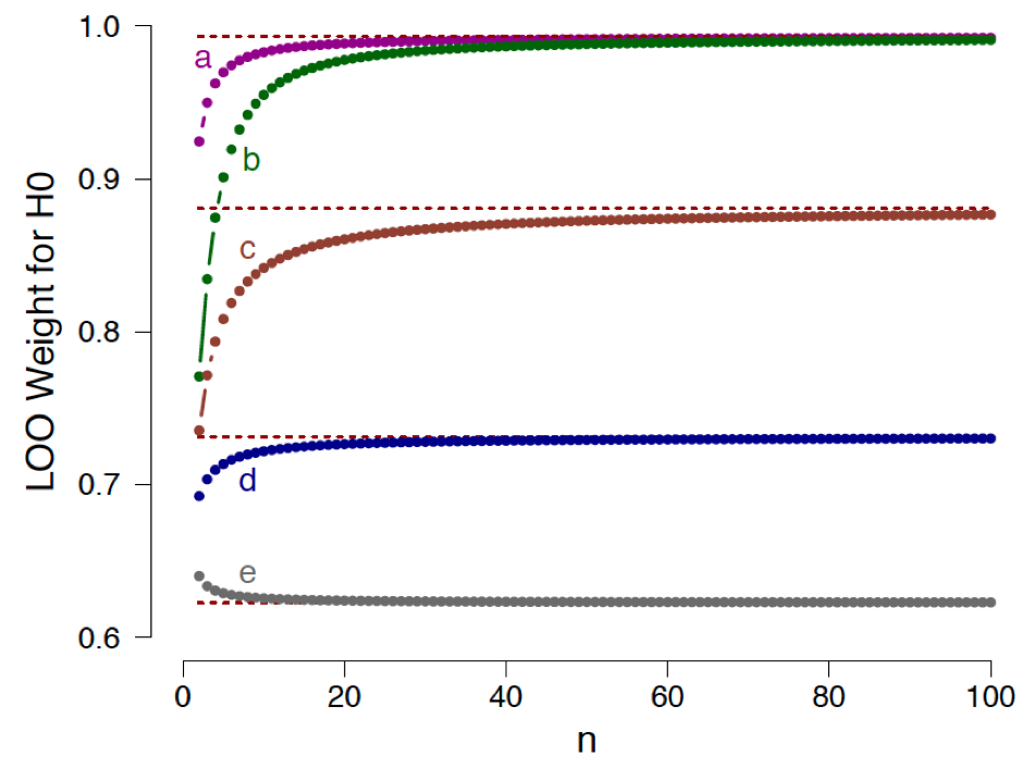
; (e)  . The dotted horizontal lines indicate the corresponding analytical asymptotic bounds. See the preprint for details. Available here under CC license.
Figure 1 shows the LOO weight in favor of the general law as a function of the number of confirmatory instances , separately for five different prior specifications under . We conclude the following: (1) as grows large, the support for the general law approaches a bound; (2) for many common prior distributions, this bound is surprisingly low. For instance, the Laplace prior  (case d) yields a weight of
  ; (3) contrary to popular belief, our results provide an example of a situation in which the results from LOO are highly dependent on the prior distribution, even asymptotically; (4) as shown by case (e) in Figure 1, the choice of Jeffreys’s prior (i.e.,
  ) results in a function that approaches the asymptote from above. This means that, according to LOO, the observation of additional confirmatory instances actually decreases the support for the general law.
Example 2: Chance
As a second example, we consider the case where the general law states that the Bernoulli rate parameter equals  rather than 1. Processes that may be guided by such a law include “the probability that a particular Uranium-238 atom will decay in the next 4.5 billion years”, or “the probability that an extrovert participant in an experiment on extra-sensory perception correctly predicts whether an erotic picture will appear on the right or on the left side of a computer screen” (Bem, 2011).
Hence, the general law holds that  , and the model that relaxes that law is given by , as in Example 1. Also, similar to Example 1, we consider the situation where the observed data are perfectly consistent with the predictions from . To accomplish this, we assume the binary data come as pairs, where one member is a success and the other is a failure.
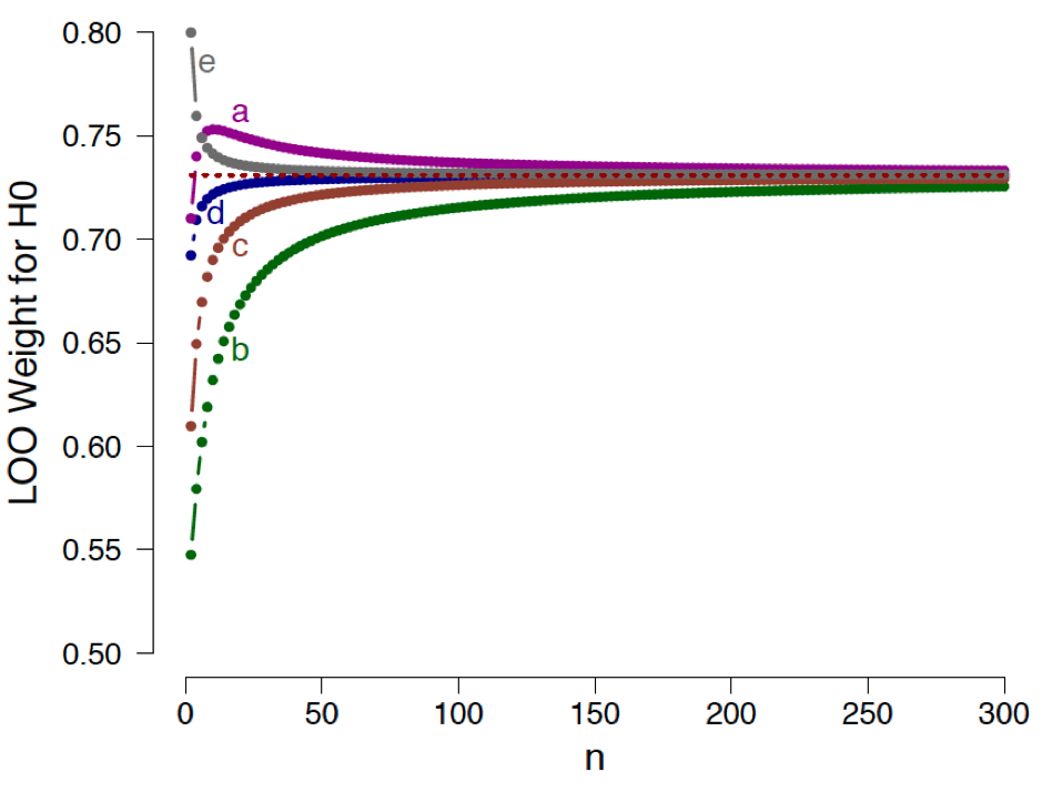
as a function of the number of observations , where the number of successes  , evaluated in relation to five different prior specifications for : (a) ; (b) ; (c) ; (d) ; (e) . The dotted horizontal line indicates the corresponding analytical asymptotic bound. Note that only even sample sizes are displayed. See the preprint for details. Available here under CC license.
Figure 2 shows the LOO weight in favor of the general law as a function of the even number of observations , separately for five different prior specifications under . We conclude the following: (1) as grows large, the support for the general law approaches a bound; (2) in contrast to Example 1, this bound is independent of the prior distribution for under ; however, consistent with Example 1, this bound is surprisingly low. Even with an infinite number of observations, exactly half of which are successes and half of which are failures, the model weight for the general law does not exceed a modest  ; (3) as shown by case (e) in Figure 2, the choice of Jeffreys’s prior (i.e., ) results in a function that approaches the asymptote from above. This means that, according to LOO, the observation of additional success-failure pairs actually decreases the support for the general law; (4) as shown by case (a) in Figure 2, the choice of a
  prior results in a nonmonotonic relation, where the addition of -consistent pairs initially increases the support for , and later decreases it.
Example 3: Nullity of a Normal Mean
As a final example, we consider the case of the  -test: data are normally distributed with unknown mean
  and known variance
  . For concreteness we consider a general law which states that the mean equals
  , that is,
  . The model that relaxes the general law assigns a zero-centered normal prior distribution with standard deviation
  . Similar to Examples 1 and 2, we consider the situation where the observed data are perfectly consistent with the predictions from . Consequently, we consider data for which the sample mean is exactly 0 and the sample variance is exactly 1.
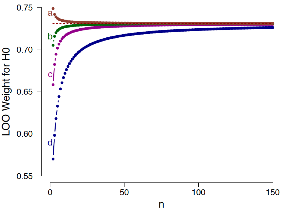
as a function of sample size , for data sets with sample mean equal to zero and sample variance equal to one, evaluated in relation to four different prior specifications for : (a)  ; (b)
; (b)  ; (c)
; (c)  ; (d)
; (d)  . The dotted horizontal line indicates the corresponding analytical asymptotic bound. See the preprint for details. Available here under CC license.
Figure 3 shows the LOO weight in favor of the general law as a function of the sample size with sample mean exactly zero and sample variance exactly one, separately for four different prior specifications of . We conclude the following: (1) as grows large, the support for the general law approaches a bound; (2) in contrast to Example 1, but consistent with Example 2, this bound is independent of the prior distribution for under ; however, consistent with both earlier examples, this bound is surprisingly low. Even with an infinite number of observations and a sample mean of exactly zero, the model weight on the general law does not exceed a modest (as in Example 2); (3) as shown by case (a) in Figure 3, the choice of a  prior distributions results in a function that approaches the asymptote from above. This means that, according to LOO, increasing the sample size of observations that are perfectly consistent with actually decreases the support for .
Conclusion
Three simple examples revealed some expected as well as some unexpected limitations of LOO. Our examples provide a concrete demonstration of the fact that LOO is inconsistent meaning that the true data-generating model will not be chosen with certainty as the sample size approaches infinity. Moreover, our examples highlighted that, as the number of -consistent observations increases indefinitely, the bound on support in favor of may remain modest. Another unexpected result was that, depending on the prior distribution, adding -consistent information may decrease the LOO preference for ; sometimes, as the -consistent observations accumulate, the LOO preference for may even be nonmonotonic, first increasing (or decreasing) and later decreasing (or increasing).
In sum, cross-validation is an appealing method for model selection. It directly assesses predictive ability, it is intuitive, and oftentimes it can be implemented with little effort. In the literature, it is occasionally mentioned that a drawback of cross-validation (and specifically LOO) is the computational burden involved. We believe that there is another, more fundamental drawback that deserves attention, namely the fact that LOO violates several common-sense desiderata of statistical support. Researchers who use LOO to adjudicate between competing mathematical models for cognition and behavior should be aware of this limitation and perhaps assess the robustness of their LOO conclusions by employing alternative procedures for model selection as well.
Like this post?
Subscribe to the JASP newsletter to receive regular updates about JASP including all its Bayesian analyses! You can unsubscribe at any time.References
Bem, D. J. (2011). Feeling the future: Experimental evidence for anomalous retroactive
influences on cognition and affect. Journal of Personality and Social Psychology, 100,
407–425.
Gronau, Q. F., & Wagenmakers, E.-J. (2018). Limitations of Bayesian leave-one-out cross-validation for model selection. Manuscript submitted for publication and available on PsyArXiv.
Lindley, D. V. (1985). Making decisions (2nd ed.). London: Wiley.
About The Authors

Quentin Gronau
Quentin is a PhD candidate at the Psychological Methods Group of the University of Amsterdam.

Eric-Jan Wagenmakers
Eric-Jan (EJ) Wagenmakers is professor at the Psychological Methods Group at the University of Amsterdam.