The Misconception

Gelman and Hennig (2017, p. 989) argue that subjective priors cannot be evaluated by means of the data:

“However, priors in the subjectivist Bayesian conception are not open to falsification (…), because by definition they must be fixed before observation. Adjusting the prior after having observed the data to be analysed violates coherence. The Bayesian system as derived from axioms such as coherence (…) is designed to cover all aspects of learning from data, including model selection and rejection, but this requires that all potential later decisions are already incorporated in the prior, which itself is not interpreted as a testable statement about yet unknown observations. In particular this means that, once a coherent subjectivist Bayesian has assessed a set-up as exchangeable a priori, he or she cannot drop this assumption later, whatever the data are (think of observing 20 0s, then 20 1s, and then 10 further 0s in a binary experiment)”
 

 
Similar claims have been made in the scholarly review paper by Consonni at al., 2018 (p. 628): “The above view of “objectivity” presupposes that a model has a different theoretical status relative to the prior: it is the latter which encapsulates the subjective uncertainty of the researcher, while the model is less debatable, possibly because it can usually be tested through data.”

The Correction

Statistical models are a combination of likelihood and prior that together yield predictions for observed data (Box, 1980; Evans, 2015). The adequacy of these predictions can be rigorously assessed using Bayes factors (Wagenmakers, 2017; but see the blog post by Christian Robert, further discussed below). In order to evaluate the empirical success of a particular subjective prior distribution, we require multiple subjective Bayesians, or a single “schizophrenic” subjective Bayesian that is willing to entertain several different priors.

Example

Only 9 years old, Emily Rosa designed a simple scientific experiment that would make her famous. The experimental setup is shown in a YouTube video here. Participants stuck their hands through two openings at the base of an opaque screen and rested them, palms up, out of view on the table at the other side. On each of 10 experimental trials, participants were asked to guess whether Emily had positioned her hand just above their left hand or just above their right hand. A towel was draped over participants’ arms in order to prevent them from peeking. The placement of Emily’s hand was determined by flipping a coin. What makes Emily’s experiment interesting is that her participants were all practicing Therapeutic Touch (TT). As summarized in the abstract of the paper that Emily later published in JAMA (The Journal of the American Medical Association), TT is “a widely used nursing practice rooted in mysticism but alleged to have a scientific basis. Practitioners of TT claim to treat many medical conditions by using their hands to manipulate a ‘human energy field’ perceptible above the patient’s skin.” (Rosa et al., 1998). In other words, TT practitioners attempt to heal illness by hovering their hands above a patient’s body and redirecting energy streams. If TT practitioners really can feel the ‘human energy field’ then they should perform above chance in Emily’s experiment. On the other hand, if their abilities are illusory then their performance in Emily’s experiment should be at chance level. Emily’s experiment was conducted in two stages. Here we focus on the first stage, which involved 15 TT practitioners. Out of the 150 decisions, only 70 were correct, for a hit rate of 46.6%, a little below chance. Clearly this is evidence against the hypothesis that the TT practitioners can feel the ‘human energy field’, but how much evidence?

For simplicity, we ignore the fact that TT practitioners may differ in their ability, and we treat all 150 trials as exchangeable. This makes the problem suitable for analysis using a straightforward binomial test that focuses on θ, the probability with which TT practitioners correctly determine the location of Emily’s hand.

As indicated in the abstract of their article, the objective of Rosa et al. was “to investigate whether TT practitioners can actually perceive a ‘human energy field’.” From the Bayesian perspective, Emily wished to assess the extent to which the data provide evidence for the skeptic’s null hypothesis (H₀: θ=1/2) that TT practitioners cannot perceive a human energy field and operate at chance accuracy versus the proponent’s alternative hypothesis (H₁: θ>1/2) that TT practitioners can perceive a human energy field and operate at above-chance accuracy.

In order for the proponent’s hypothesis to be tested against data, the hypothesis must make predictions, and this requires that the success probability parameter θ be assigned a prior distribution. Here we distinguish three different proponents who each specify their own subjective distribution. Our first proponent comes from Mars, and specifies (“any success rate is equally likely; the value of 1/2 does not receive special attention”). Our second proponent is conservative, and specifies (“success rates are higher than 0.5, but those near 0.5 are much more likely than those near 1; the value of 1/2 does not receive special attention other than as a lower bound). Finally, our third proponent is optimistic and specifies (“success rates are higher than 0.5, and those near 0.75 are more likely than those near 0.5 or near 1; the value of 1/2 does not receive special attention other than as a lower bound).

We will start by comparing the skeptic’s position to each of the proponents’ positions. We do this by comparing their predictive adequacy for the data observed, which, in Emily Rosa’s case, equals 70 correct decisions out of 150 attempts (i.e., at 46.7%, performance in the sample is a little lower than chance).

First, we compare the skeptic’s position to that of the proponent from Mars. The resulting inference is summarized in the prior-posterior plot from JASP:

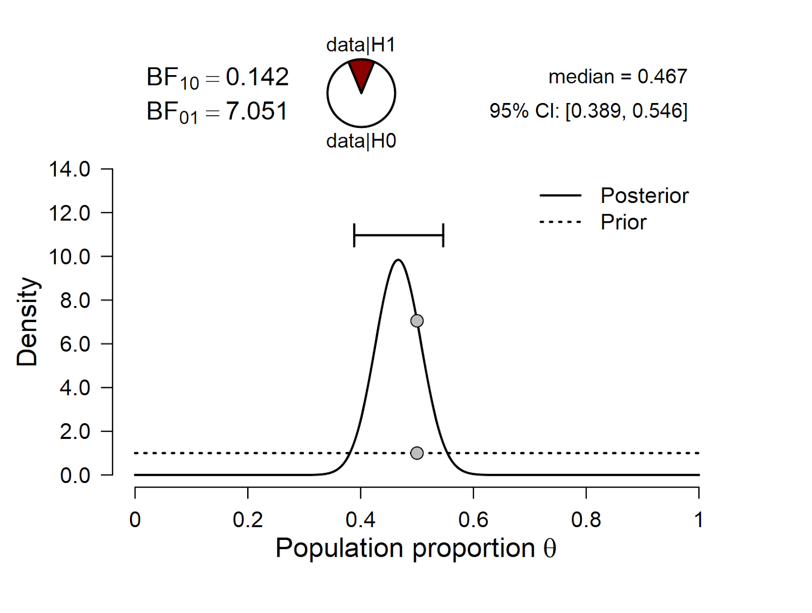
Figure 1. Skeptic vs. proponent from Mars.

The results show that BF₀₁ = 7.051, that is, the skeptic’s null hypothesis outpredicts the proponent from Mars by a factor of about 7.

Next we compare the skeptic’s position to that of the conservative proponent:

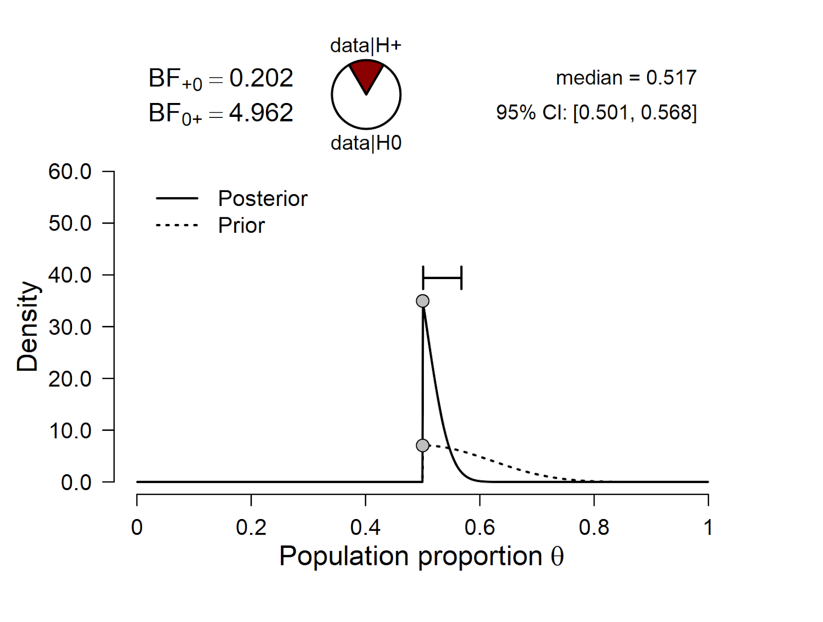
Figure 2. Skeptic vs. conservative proponent.

The results show that BF₀₁ = 4.962, that is, the skeptic’s null hypothesis outpredicts the conservative proponent by a factor of about 5.

Finally, we compare the position of the skeptic against that of the optimistic proponent:

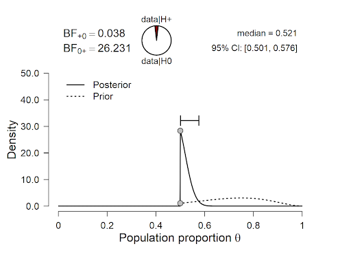
Figure 3. Skeptic vs. optimistic proponent.

The results show that BF₀₁ = 26.231, that is, the skeptic’s null hypothesis outpredicts the optimistic proponent by a factor of about 26.

It is clear that, although the null hypothesis outpredicts all three of the proponent hypotheses, it does so with varying degrees of decisiveness. Denoting the skeptic’s null hypothesis by S, the Mars proponent hypothesis by M, the conservative proponent hypothesis by C, and the optimistic proponent hypothesis by O, we have:

BF_SM = 7.051
BF_SC = 4.962
BF_SO = 26.231

These Bayes factors are ratios that all involve the skeptics hypothesis S; consequently, dividing one Bayes factor by another makes S drop out, and what remains is a Bayes factor that compares the predictive adequacy of two proponent hypotheses, that is, the adequacy of their prior distributions. Specifically, we have

BF_SM / BF_SC = BF_SM * BF_CS = BF_CM which evaluates to 7.051 / 4.962 = 1.421. This means that the prior from the conservative proponent predicted the data better than the prior from the Mars proponent, although the predictive advantage is minute.

In the same vein, we find that BF_SO / BF_SC = BF_SO * BF_CS = BF_CO which evaluates to 26.231 / 4.962 5.286, that is, the prior from the conservative proponent outpredicts the prior from the optimistic proponent by a factor of about 5. This predictive advantage is moderate — if the conservative and optimistic perspectives were equally likely a priori, the data would increase the probability for the conservative position from a prior value of .50 to a posterior value of .84, which still leaves a posterior probability of .16 for the optimistic position.

Finally, we may compute that BF_SO / BF_SM = BF_SO * BF_MS = BF_MO which evaluates to 26.231 / 7.051 3.72: just as the conservative proponent, the Mars proponent outperforms the optimistic proponent, but the predictive advantage for the Martian is not large — the data would increase a prior model probability of .50 to .79, leaving .21 to the optimistic perspective.

The above example demonstrates how the Bayes factor quantifies the relative predictive adequacy of the different subjective prior distributions. This should not come as a surprise: a prior distribution may be considered a bet on the different values that the parameter can take on, and the whole purpose of a bet is to be evaluated against data.

Want to Know More?

Alternative methods to assess the extent to which the information in the data conflicts with the prior distribution are discussed by Box (1980), and references therein. A more recent treatment of the topic can be found in the chapter “Choosing and Checking the Model and Prior,” by Evans (2015). Finally, Christian Robert has explicitly argued against the use of Bayes factors for comparing prior distributions ; we agree with Christian Robert’s factual statements (specifically, we agree that, under regularity conditions, the Bayes factor between two continuous priors will approach a bound as the data set increases indefinitely; for an empirical demonstration see Gronau & Wagenmakers, 2018) but we are not swayed by some of his other arguments. Specifically, the goal of the Bayes factor comparison of priors, as we envision it here, is not to select a prior and then use that prior a second time to analyze the data to draw conclusions (this would be double-dipping, as Christian Robert is right to point out), but rather to decide which prior distribution yields the best predictive performance and leave it at that. Note that this is the usual purpose of the Bayes factor, to grade the evidence for the skeptic’s point prior distribution versus the proponent’s bell-shaped prior distribution; the comparison between multiple bell-shaped priors follows directly from transitivity, as was shown in the therapeutic touch example above.

References

Box, G. E. P. (1980). Sampling and Bayes’ inference in scientific modelling and robustness. Journal of the Royal Statistical Society, Series A, 143, 383-430.

Consonni, G., Fouskakis, D., Liseo, B., Ntzoufras, I. (2018). Prior distributions for objective Bayesian analysis. Bayesian Analysis, 13, 627-679.

Evans, M. (2015). Measuring statistical evidence using relative belief. Boca Raton, FL: CRC Press.

Gelman, A., & Hennig, C. (2017). Beyond subjective and objective in statistics. Journal of the Royal Statistical Society Series A, 180, 967-1033.

Gronau, Q. F., & Wagenmakers, E.-J. (2018). Bayesian evidence accumulation in experimental mathematics: A case study of four irrational numbers. Experimental Mathematics, 27, 277-286.

Rosa, L., Rosa, E., Sarner, L., & Barrett, S. (1998). A close look at therapeutic touch. The Journal of the American Medical Association, 279, 1005-1010.

Wagenmakers, E.-J. (2017). Comment on Gelman and Hennig, “Beyond subjective and objective in statistics”. Journal of the Royal Statistical Society Series A, 180, 1023.

About The Author

Quentin Gronau

Quentin is a PhD candidate at the Psychological Methods Group of the University of Amsterdam.

Eric-Jan Wagenmakers

Eric-Jan (EJ) Wagenmakers is professor at the Psychological Methods Group at the University of Amsterdam.