This post is a teaser for
Wagenmakers, E.-J. (2022). Approximate objective Bayes factors from p-values and sample size: The 3p√n rule. Preprint available on ArXiv: https://psyarxiv.com/egydq
Abstract
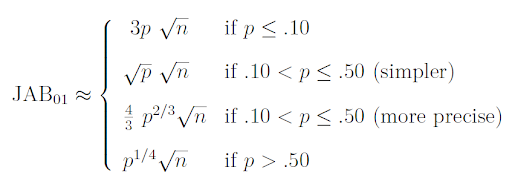
“In 1936, Sir Harold Jeffreys proposed an approximate objective Bayes factor that quantifies the degree to which the point-null hypothesis H0 outpredicts the alternative hypothesis H1. This approximate Bayes factor (henceforth JAB01) depends only on sample size and on how many standard errors the maximum likelihood estimate is away from the point under test. We revisit JAB01 and introduce a piecewise transformation that clarifies the connection to the frequentist two-sided p-value. Specifically, if p ≤ .10 then JAB01 ≈ 3p√n; if .10 < p ≤ .50 then
JAB01 ≈ √(pn); and if p > .50 then JAB01 ≈ p^(¼)√n. These transformation rules present p-value practitioners with a straightforward opportunity to obtain Bayesian benefits such as the ability to monitor evidence as data accumulate without reaching a foregone conclusion. Using the JAB01 framework we derive simple and accurate approximate Bayes factors for the t-test, the binomial test, the comparison of two proportions, and the correlation test.”
Summary in Figures
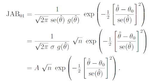
This is Jeffreys’s general expression for the Bayes factor in favor of the null hypothesis:
Using the p-value transformations we obtain the following approximate relations:
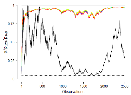
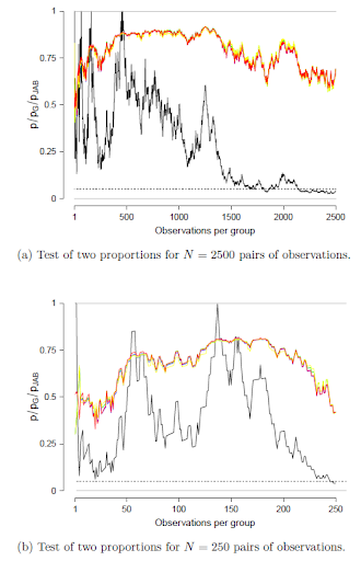
When applied to popular tests, the results closely approximate those from default Bayes factors. For instance, here is an example application to a test between two proportions, where a sequence of observations is generated under the null hypothesis; the black line shows the fixed-N p-value, which drifts randomly as sample size grows; the colors indicate posterior probabilities for the null hypothesis computed using different Bayesian methods, including the exact default Bayes factor proposed by Kass & Vaidyanathan, 1992, implemented by Gronau et al., 2021, and tutorialized by Hoffmann et al., 2021):
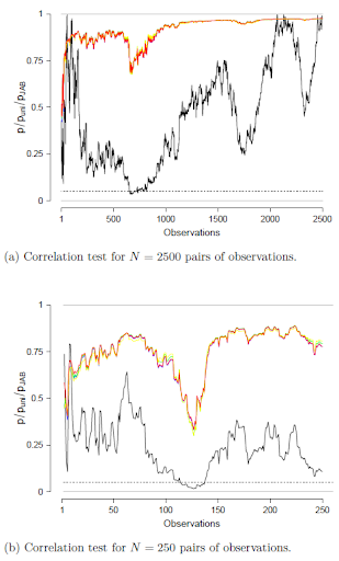
And this shows a similar example, now for the Pearson correlation test:
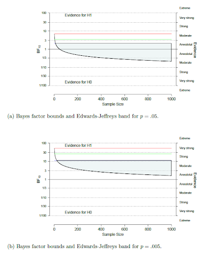
The Edwards-Jeffreys Bayes Factor Band
Researchers who question the unit-information prior that underlies Jeffreys’s simple Bayes factor may instead report a band of Bayes factors, one that ranges from the result obtained by Jeffreys to an upper bound obtained by Edwards et al. (1963), that is, a Bayes factor based on a normal prior distribution centered on the point at test, and with variance cherry-picked to yield the strongest evidence against the null hypothesis. The azure band in the top panel is for p=.05 results, and in the bottom panel it is for p=.005 results.
References
Edwards, W., Lindman, H., & Savage, L. J. (1963). Bayesian statistical inference for psychological research. Psychological Review, 70, 193-242.
Gronau, Q. F., Raj, K. N. A., & Wagenmakers, E.-J. (2021). Informed Bayesian inference for the A/B test. Journal of Statistical Software, 100, 1-39. Url: https://www.jstatsoft.org/article/view/v100i17
Hoffmann, T., Hofman, A., & Wagenmakers, E.-J. (2021). A tutorial on Bayesian inference for the A/B test with R and JASP. Manuscript submitted for publication. Preprint: https://psyarxiv.com/z64th
Kass, R. E., & Vaidyanathan, S. K. (1992). Approximate Bayes factors and orthogonal parameters, with application to testing equality of two binomial proportions. Journal of the Royal Statistical Society, Series B, 54, 129-144.
Wagenmakers, E.-J., & Ly, A. (2021). History and nature of the Jeffreys-Lindley paradox. Manuscript submitted for publication. Preprint: https://arxiv.org/abs/2111.10191
About The Author

Eric-Jan Wagenmakers
Eric-Jan (EJ) Wagenmakers is professor at the Psychological Methods Group at the University of Amsterdam.