This post is a teaser for Wagenmakers, E.-J., & Ly, A. (2020). History and nature of the Jeffreys-Lindley paradox. Preprint available on ArXiv: https://arxiv.org/abs/2111.10191

Abstract

“The Jeffreys-Lindley paradox exposes a rift between Bayesian and frequentist hypothesis testing that strikes at the heart of statistical inference. Contrary to what most current literature suggests, the paradox was central to the Bayesian testing methodology developed by Sir Harold Jeffreys in the late 1930s. Jeffreys showed that the evidence against a point-null hypothesis H0 scales with √n and repeatedly argued that it would therefore be mistaken to set a threshold for rejecting H0 at a constant multiple of the standard error. Here we summarize Jeffreys’s early work on the paradox and clarify his reasons for including the √n term. The prior distribution is seen to play a crucial role; by implicitly correcting for selection, small parameter values are identified as relatively surprising under H1. We highlight the general nature of the paradox by presenting both a fully frequentist and a fully Bayesian version. We also demonstrate that the paradox does not depend on assigning prior mass to a point hypothesis, as is commonly believed.”

Jeffreys Did it First, and Better

“Contrary to popular belief, our analysis reveals that the paradox played a central role in Jeffreys’s system of Bayes factor hypothesis tests, and did so from the outset. (…) The common notion that Jeffreys mentioned the paradox only in passing is therefore seriously incorrect.”

“For over two decades, Jeffreys had repeatedly pointed out the potential conflict between p-values and Bayes factors. However, Jeffreys’s work on Bayes factors had been largely ignored. Instead, it was the 1957 article by Lindley that brought the paradox into the limelight. (…)

Based on our reading, we conclude that both Lindley and Bartlett unwittingly presented a slightly confused version of Jeffreys’s earlier work. (…)

In sum, the arguments presented in Lindley (1957) and Bartlett (1957) were already discussed two decades earlier by Jeffreys, in more detail and without errors.”

A Fully Frequentist Version of the Paradox

“Thus, if the prior distribution is calibrated then the Bayes factor provides an optimal frequentist decision criterion. This also holds when the frequentist purpose is to minimize a weighted sum of errors, λα + β (Cornfield, 1966). Thus, from a Neyman-Pearson perspective, the conflict with a Bayesian assessment of evidence arises specifically in the common scenario where the researcher fixes the probability of a Type I error (say to 5%) and then tries to minimize the probability  of a Type II error. However, as pointed out above, in high-n situations the researcher may prefer to sacrifice some power in order to lower the probability of a Type I error. As indicated above Egon Pearson himself judged this strategy “quite legitimate” (Pearson, 1953, p. 69). Applying this strategy substantially reduces the discrepancy between the frequentist and the Bayesian results.”

“In sum, the Jeffreys-Lindley paradox may be given a purely frequentist interpretation as a discrepancy between (a) minimizing β for fixed α; versus (b) minimizing the weighted sum of errors, λα + β.”

A Fully Bayesian Version of the Paradox

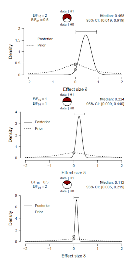
“The relation between the one-sided p-value and the Bayesian test for direction suggests that the Jeffreys-Lindley paradox can be given a fully Bayesian interpretation. Specifically, data may be constructed which will convince the Bayesian that the population effect is positive rather than negative (…), whereas this same Bayesian will also be convinced that the population effect is absent rather than present. (…) This state of knowledge is not incoherent, but it may be counter-intuitive.”

The scenario is illustrated in the figure below. Each panel shows the prior and posterior for effect size in a t-test. All panels have the same posterior mass on negative effect size and therefore offer the same evidence that the effect is positive rather than negative (i.e., BF+− = 47.9768). At the same time, the test against the point-null hypothesis H0 reveals increasing support for H0 as sample size n grows (top: n = 20; middle: n = 82; bottom: n = 332).

A First Attempt to Escape from the Paradox: Down with Point Masses!

“One attempt to question the relevance of the paradox is to argue that the null hypothesis is never true exactly, and it is unwise to assign separate prior mass to a single point from a continuous distribution.”

“The impression that the paradox arises because H0 has separate prior mass is strengthened by Jeffreys’s own work.”

However,

“(…) the paradox does not require the presence of a point-null hypothesis. This fact is almost universally overlooked (for an exception see Cousins, 2017).”

“The peri-null does not include point masses; yet, the Jeffreys-Lindley paradox still applies.”

“In sum, the Jeffreys-Lindley paradox does not depend on the presence of a point-null hypothesis, as is usually claimed. For fixed p = α, the data will inevitably support a peri-null hypothesis over the alternative hypothesis as sample size grows large. The strength of this support is bounded, but in favor of the peri-null, thus leaving the conflict qualitatively intact. In other words, even when the point-null is replaced by a peri-null hypothesis, “there would be cases, with large numbers of observations, when a new parameter is asserted on evidence that is actually against it.” (Jeffreys, 1938a, pp. 379).”

A Second Attempt to Escape from the Paradox: Blaming the Prior

“Whenever the paradox occurs, a natural objection to the Bayes factor outcome is that the prior distribution for the test-relevant parameter under H1 was too wide, wasting considerable prior mass on large values of effect size that yield poor predictive performance. Thus, as implied by Bartlett (1957), the paradox reveals a fault in the specification of H1 rather than H0.

“In general terms, the critique that the prior was too wide is made post-hoc; after observing a near-zero effect size one may always argue that, in hindsight, the prior was too wide – if such reasoning were allowed then the data could never undercut H1 and support H0. As long as the prior width does not shrink as a function of sample size, the paradox arises under any non-zero prior width.”

Main Conclusions

“In this paper we examined the history and nature of the Jeffreys-Lindley paradox.

Our main conclusions are as follows:

1. Contrary to what the current literature suggest (e.g., Bernardo & Smith, 2000, p. 394; O’Hagan & Forster, 2004, p. 78), the Jeffreys-Lindley paradox was central to Harold Jeffreys’s philosophy of Bayesian testing; in Jeffreys’s tests, the critical threshold is not based on a constant multiple of the standard error but instead involves a n term.
2. From 1935 to 1936, Jeffreys had discovered, understood, published, emphasized, explained, and illustrated the paradox. It remained a recurring theme throughout his later articles and books.
3. The articles by Lindley (1957) and Bartlett (1957) echo earlier work by Jeffreys. This is acknowledged by both authors, but they do not seem fully aware of the extent to which Jeffreys had already studied the issue. The two 1957 articles also introduced some mathematical errors and conceptual misunderstandings.
4. The paradox is caused by the fact that, as n increases and p remains constant, an ever increasing set of parameter values under H1 is inconsistent with the observed data, decreasing H1’s average predictive performance (i.e., the marginal likelihood).
5. A fully frequentist version of the paradox contrasts the inductive behavior of two frequentists, one who fixes α and minimizes β, the other who minimizes a weighted linear sum of α and β (e.g., Cornfield, 1966; Lehmann, 1958; Lindley, 1953). As n grows large, the same data that prompt the former frequentist to reject H0 will prompt the latter frequentist to retain H0. The behavior of the latter frequentist is qualitatively consistent with the tests proposed by Jeffreys.
6. A fully Bayesian version of the paradox contrasts the beliefs of two Bayesians, one who tests H+: δ > 0 versus H− : δ < 0 (i.e., the direction of the effect), the other who tests H0 : δ = 0 versus H1 :  δ ≠ 0 (i.e., the presence of the effect). As n grows large, the same data that prompt the former Bayesian to conclude that the data offer strong support for the hypothesis that the effect is positive will prompt the latter Bayesian to conclude that the data offer strong support for the hypothesis that the effect is absent.
7. Contrary to what the current literature suggests, the root of the paradox is not in the assignment of prior mass to a point hypothesis H0; the paradox is also present when the point-null hypothesis is replaced by a peri-null hypothesis (i.e., a relatively peaked continuous distribution).
8. The Jeffreys-Lindley paradox is relatively robust: it holds whether or not H0 is a point-null or a peri-null hypothesis, and it holds regardless of the width of the prior distribution for the test-relevant parameter under H1 – as long as the width is larger than that of the prior distribution under the peri-null hypothesis, and as long as it does not shrink with sample size.
9. The Jeffreys-Lindley paradox results from the discrepancy between two modes of inference: (1) evaluating a single model (e.g., fixed-α decision making); (2) contrasting two models, one of which is relatively simple (e.g., the skeptic’s H0) and one which is more complex (e.g., the proponent’s H1).”

Finishing Up

“Would Jeffreys have endorsed the recent proposal to reduce the significance level for new discoveries from α = .05 to α = .005 (Benjamin et al., 2018)? We believe he would have had reservations. Although the proposal was motivated in part by Bayesian insights that originate from Jeffreys himself, the stricter α level still entails a threshold that is a constant multiple of the standard error and omits the crucial √n term. Moreover, endorsing the α = .005 proposal would mean an implicit admission that his repeated reassurances concerning the use of
α = .05 as “about right” were in fact wrong.

A thorough understanding of the Jeffreys-Lindley paradox remains critically important for the assessment of statistical methodology, both old and new. Ultimately, the paradox may even bring about some reconciliation between the Bayesian and the frequentist frameworks – in particular, the paradox may motivate frequentists to explore procedures that minimize the weighted sum of α and β, which ought to yield conclusions similar to those obtained with Jeffreys’s Bayesian tests (cf. Lindley, 1953; Pericchi & Pereira, 2016). We believe this manuscript provides some new historical and conceptual background to the Jeffreys-Lindley paradox, and we hope that this will be useful for statistical theory as well as statistical practice.”

References

Wagenmakers, E.-J., & Ly, A. (2021). History and nature of the Jeffreys-Lindley paradox. Manuscript submitted for publication. ArXiv preprint: https://arxiv.org/abs/2111.10191

About The Authors

Eric-Jan Wagenmakers

Eric-Jan (EJ) Wagenmakers is professor at the Psychological Methods Group at the University of Amsterdam.

Alexander Ly

Alexander Ly is a postdoc at the Psychological Methods Group at the University of Amsterdam.