“Anything is fair in love and war” — this saying also applies to the eternal struggle between frequentists (those who draw conclusions based on the performance of their procedures in repeated use) and Bayesians (those who quantify uncertainty for the case at hand). One argument that frequentists have hurled at the Bayesian camp is that “Bayesian procedures do not control error rate”. This sounds like a pretty serious accusation, and it may perhaps dissuade researchers who are on the fence from learning more about Bayesian inference. “Perhaps,” these researchers argue, “perhaps the Bayesian method for updating knowledge is somehow deficient. After all, it does not control error rate. This sounds pretty scary”.
The purpose of this post is twofold. First, we will show that Bayesian inference does something much better than “controlling error rate”: it provides the probability that you are making an error for the experiment that you actually care about. Second, we will show that Bayesian inference can be used to “control error rate” — Bayesian methods usually do not strive to control error rate, but this is not because of a some internal limitation; instead, Bayesians believe that it is simply more relevant to know the probability of making an error for the case at hand than for imaginary alternative scenarios. That is, for inference, Bayesians adopt a “post-data” perspective in which one conditions on what is known. But it is perfectly possible to set up a Bayesian procedure and control error rate at the same time.
Schmerror Rate
You are running an elk taxidermy convention in Finland, and you wish to know whether the participants find the conference rooms too hot or too cold. You decide to ask a few participants for their opinion: do they find the rooms too hot or too cold? Inference concerns the binomial rate parameter  ; if you’ve set the temperature just right then half of the people will find the room too hot, and half will find it too cold (i.e., the null hypothesis states that
  ). Out of the first ten participants you ask, nine indicate the rooms are too cold, and a single one indicates the rooms are too hot.
We can easily conduct a frequentist analysis in JASP. The figure below shows the data panel to the left, the analysis input panel in the middle, and the output panel to the right. Let’s focus on the first row of the table in the output panel, which involves the test that compares the answer “TooCold” to anything else (which, in this case, happens to be the only alternative answer, “TooHot”). We can see that the proportion “TooCold” responses in the sample is 90%. The two-sided p-value is .021 and the 95% confidence interval ranges from 0.555 to 0.997. Let’s pause a minute to reflect on what this actually means.
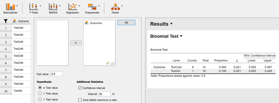
First, the p-value is the probability of encountering a test statistic at least as extreme as the one that is observed, given that the null hypothesis is true. In this case, a natural test statistic (i.e., a summary of the data) is the total number of “TooCold” responses. So in this case the value of the observed test statistic equals 9. The cases that are at least as extreme as “9” are “9” and “10”. Because we are conducting a two-sided test, we also need to consider the extreme cases at the other end of the sampling distribution, that is, “0” and “1”. So in order to obtain the coveted p-value, we sum four probabilities: Pr(0 out of 10 | H0), Pr(1 out of 10 | H0), Pr(9 out of 10 | H0), and Pr(10 out of 10 | H0). Now that we’ve computed the holy p-value, what shall we do with it? Well, this is surprisingly unclear. Fisher, who first promoted their use, viewed low p-values as evidence against the null-hypothesis. Here we follow his nemeses Neyman and Pearson, however, and employ a different framework, one that focuses on performance of the procedure in the long run. Assume we set a threshold  , and we “reject the null hypothesis” whenever our p-value is lower than . The most common value of is .05. As an aside, some people have recently argued that one ought to justify a specific value for ; now justifying something is always better than not justifying it, but it seems to us that when you are going to actually think about statistics then it is more expedient to embrace the Bayesian method straight away instead of struggling with a set of procedures whose main attraction is the mindlessness with which they are applied.
Anyhow, the idea is that the routine use of a Neyman-Pearson procedure controls the “Type I error rate” at ; what this means is that if the procedure is applied repeatedly, to all kinds of different data sets, and the null hypothesis is true, the proportion of data sets for which the null hypothesis will be falsely rejected is lower or equal to . Crucially, “proportion” refers to hypothetical replications of the experiment with different outcomes. Suppose we find that  . We can then say: “We rejected the null hypothesis based on a procedure that, in repeated use, falsely rejects the null hypothesis in no more than 5% of the hypothetical experiments.” As an aside, the 95% confidence interval is simply the collection of values that would not be rejected at an level of 5% (for more details see Morey et al., 2016).
Note that the inferential statement refers to performance in the long run. Now it is certainly comforting to know that the procedure you are using does well in the long-run. If one could tick one of two boxes, “your procedure draws the right conclusion for most data sets” or “your procedure draws the wrong conclusion for most data sets” then –all other things being equal– you’d prefer the first option. But Bayesian inference has set its sights on a loftier goal: to infer the probability of making an error for the specific data set at hand.
Before we continue, it is important to stress that Neyman-Pearson procedures only control the error rate conditional on the null hypothesis being true. This is arguably less relevant than the error rate conditional on the decision that was made. Suppose you conduct an experiment on the health benefits of homeopathy and find that p=.021. You may feel pretty good about rejecting the null, but it is misleading to state that your error rate for this decision is 5%; assuming that homeopathy is ineffective, your error rate among experiments in which you reject the null hypothesis is 100%.
The Probability of Making an Error
We analyze the above taxidermy data set in JASP using the Bayesian binomial test. The key output is as follows:
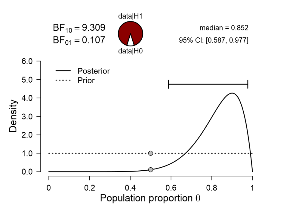
The dotted line is the prior distribution. JASP allows different prior distributions to be specified, but for the taxidermy example this distribution is not unreasonable. Ultimately this is an interesting modeling question, just like the selection of the binomial likelihood (for more details see Lee & Vanpaemel, 2018; Lee, in press). The solid line is the posterior distribution. If no single value of is worthy of special consideration, we can be 95% confident that the true value of falls between 0.587 and 0.977. Note that this interval does not refer to hypothetical replications of the experiment, as does the frequentist confidence interval: instead, it refers to our confidence about this specific scenario. A similar case-specific conclusion can be drawn when we assume that there is a specific value of that warrants special attention; in this case, we may compare the predictive performance of the null hypothesis  against that of the alternative hypothesis
  (i.e., the uniform prior distribution shown above). The result shows that the Bayes factor equals 9.3 in favor of H1; that is, the data are 9.3 times more likely under H1 than under H0. This does not give us the probability of making an error. To obtain this probability, we need to make an assumption about the prior plausibility of the hypotheses. When we assume that both hypotheses are equally likely a priori, the posterior probability of H1 is 9.3/10.3 = .90, leaving .10 posterior probability for H0. So here we have the first retort to the accusation that “Bayesian methods do not control error rate”: Bayesian methods achieve a higher goal, namely the probability of making an error for the case at hand. In the taxidermy example, the probability of making an error if H0 is “rejected” is .10.
Three remarks are in order. First, in academia we rarely see the purpose of an all-or-none “decision”, and in statistics we can rarely be 100% certain. In some situation there is action to be taken, but in research the action is often simply the communication of the evidence, and for this one does not need to throw away information by impoverishing the evidence space into “accept” and “reject” regions. Second, if action is to be taken and the evidence space needs to be discretized, then it is imperative to specify utilities (see Lindley, 1985, for examples). So the full treatment of a decision problem requires utilities, prior model probabilities, and prior distributions for the parameters within the models. It should be evident that the rule “reject H0 whenever  ” is way, way too simplistic an approach for the problem of making decisions. Finally, if you seek to make an all-or-none decision, the Bayesian paradigm yields the probability that you are making an error. With this probability in hand, it is not immediately clear why one would be interested in the probability of making an error averaged across imaginary data sets that differ from the one that was observed. But because it is not of interest to compute a certain number does not mean it cannot be done.
Error Rate of Bayesian Procedures
Would a Bayesian ever be interested in learning about the hypothetical outcomes for imaginary experiments? The answer is “yes, but only in the planning stage of the experiment”. In the planning stage, no data have yet been observed, and, taking account of all uncertainty, the Bayesian needs to average across all possible outcomes of the intended experiment. So before the experiment is conducted, the Bayesian may be interested in “pre-data inference”; for instance, this may include the probability that a desired level of evidence will be obtained before the resources are depleted, or the probability of obtaining strong evidence for the null hypothesis with a relatively modest sample size, etc. However, as soon as the data have been observed, the experimental outcome is not longer uncertain, and the Bayesian can condition on it, seamlessly transitioning to “post-data” inference. The Bayesian mantra is simple: “condition on what you know, average across what you don’t”.
Nevertheless, in the planning stage the Bayesian can happily compute error rates, that is, probabilities of obtaining misleading evidence (see Schönbrodt & Wagenmakers, 2018; Schönbrodt, Wagenmakers, Zehetleitner, & Perugini, 2017; Stefan et al., 2018; see also Angelika’s fabulous planning app here
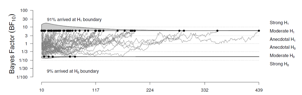
Or one may adopt a fixed-N design and examine the distribution of expected Bayes factors, tallying the proportion of them that go in the “wrong direction” (e.g., the proportion of expected Bayes factors that strongly support H1 even though the data were generated under H0). When the actual data are in, it would be perfectly possible to stick to the “frequentist” evaluation and report the “error rate” of the procedure across all data that could have materialized. And if this is what gets you going, by all means, report this error rate. But with two error rates available, it seems to us that the most relevant one is the probability that you are making an error, not the proportion of hypothetical data sets for which your procedure reaches an incorrect conclusion.
In sum:
References
Lee, M. D., & Vanpaemel, W. (2018). Determining informative priors for cognitive models. Psychonomic Bulletin & Review, 25, 114-12.
Lee, M. D. (in press). Bayesian methods in cognitive modeling. In Wixted, J. T., & Wagenmakers, E.-J. (Eds.), Stevens’ Handbook of Experimental Psychology and Cognitive Neuroscience (4th ed.): Volume 4: Methodology. New York: Wiley.
Lindley, D. V. (1985). Making Decisions (2nd ed.). London: Wiley.
Morey, R. D., Hoekstra, R., Rouder, J. N., Lee, M. D., & Wagenmakers, E.-J. (2016). The fallacy of placing confidence in confidence intervals. Psychonomic Bulletin & Review, 23, 103-123. For more details see Richard Morey’s web resources.
Schönbrodt, F. D., Wagenmakers, E.-J., Zehetleitner, M., & Perugini, M. (2017). Sequential hypothesis testing with Bayes factors: Efficiently testing mean differences. Psychological Methods, 22, 322-339.
Schönbrodt, F., & Wagenmakers, E.-J. (2018). Bayes factor design analysis: Planning for compelling evidence. Psychonomic Bulletin & Review, 25, 128-142. Open Access.
Stefan, A. M., Gronau, Q. F., Schönbrodt, F. D., & Wagenmakers, E.-J. (2018). A tutorial on Bayes factor design analysis with informed priors. Manuscript submitted for publication.
About The Authors

Eric-Jan Wagenmakers
Eric-Jan (EJ) Wagenmakers is professor at the Psychological Methods Group at the University of Amsterdam.

Quentin Gronau
Quentin is a PhD candidate at the Psychological Methods Group of the University of Amsterdam.