Bayesian inference offers the pragmatic researcher a series of perks (Wagenmakers, Morey, & Lee, 2016). For instance, Bayesian hypothesis tests can quantify support in favor of a null hypothesis, and they allow researchers to track evidence as data accumulate (e.g., Rouder, 2014).
However, Bayesian inference also confronts researchers with new challenges, for instance concerning the planning of experiments. Within the Bayesian paradigm, is there a procedure that resembles a frequentist power analysis? (yes, there is!)
In this blog post, we explain Bayes Factor Design Analysis (BFDA; e.g., Schönbrodt & Wagenmakers, in press), and describe an interactive web application that allows you to conduct your own BFDA with ease. If you want to go straight to the app you can skip the next two sections; if you want more details you can read our PsyArXiv preprint.
What is a Bayes Factor Design Analysis (BFDA)?
As the name implies, Bayes Factor Design Analysis provides information about proposed research designs (Schönbrodt & Wagenmakers, in press). Specifically, the informativeness of a proposed design can be studied using Monte Carlo simulations: we assume a population with certain properties, repeatedly draw random samples from it, and compute the intended statistical analyses for each of the samples. For example, assume a population with two sub-groups whose standardized difference of means equals δ = 0.5. Then, we can draw 10,000 samples with N = 20 observations per group from this population and compute a Bayesian t-test for each of the 10,000 samples. This procedure will yield a distribution of Bayes factors which you can use to answer the following questions:
- Which evidence strength can I expect for this specific research design?
- Which rates of misleading evidence can I expect for this research design given specific evidence thresholds?
The figure below shows the distribution of default Bayes factors for the research design from our example using evidence thresholds of ⅙ and 6. This means that Bayes factors smaller than ⅙ are considered as evidence for the null hypothesis and Bayes factors larger than 6 are considered as evidence for the alternative hypothesis. Note that the only function of these thresholds is to be able to define “error rates” (rates of misleading evidence) and appease frequentists who worry that the Bayesian paradigm does not control these error rates. Ultimately though, the Bayes factor is what it is, regardless of how we set the thresholds. From Figure 1, you can see that the proposed research design yields about 0.4% false negative evidence (BF10 < ⅙) and 20.1% true positive evidence (BF10 > 6). This means that in almost 80% of the cases the Bayes factor will be stranded in no man’s land.
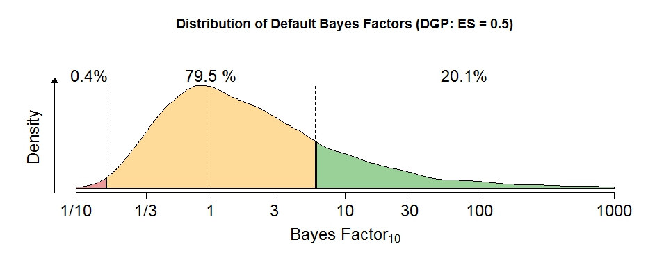
Figure 1: Distribution of Bayes Factors for a data generating process (DGP) of δ = 0.5 in a one-sided independent-samples t-test with n = 20 per group.
BFDA for Sequential Designs
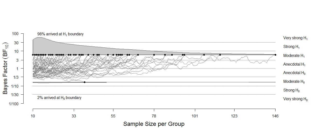
In sequential designs, researchers can use a rule to decide, at any stage of the experiment, whether (1) to accept the hypothesis being tested; (2) to reject the hypothesis being tested; or (3) to continue the experiment and collect additional observations (Wald, 1945). In sequential hypothesis testing with Bayes factors (Schönbrodt et al., 2017), the decision rule can be based on the obtained strength of evidence. For example, a researcher might aim for a strength of evidence of 6 and thus collect data until the Bayes factor is larger than 6 or smaller than ⅙.
This implies that in sequential designs, the exact sample size is unknown prior to conducting the experiment. However, it may still be useful to assess whether you have sufficient resources to complete the intended experiment. For example, if you want to pay participants €10 each, will you likely need €200, €2000, or €20,000? If you don’t want to go bankrupt, it is good to plan ahead. [As an aside, a Bayesian should feel uninhibited to stop the experiment for whatever reason, including impending bankruptcy. But, as indicated above, by specifying a stopping rule in advance we are able to “control” the rate of misleading evidence].
Given certain population effects and decision rules, a sequential BFDA provides a distribution of sample sizes, indicating the number of participants that are needed to reach a target level of evidence. The sequential BFDA can also be used to predict the rates of misleading evidence, that is: How often will the Bayes factors arrive at the “wrong” evidence threshold?
The BFDA App
In order to make it easy to conduct a BFDA, we developed an BFDA App.
Currently, the app allows you to conduct a BFDA for one-sided t-tests with two different priors on effect size: a “default” prior as implemented in the BayesFactor R package (Morey & Rouder, 2015; Cauchy(µ = 0, r = 2/2)) and an example “informed” prior, that is, a shifted and scaled t-distribution elicited for a social psychology replication study (Gronau, Ly, & Wagenmakers, 2017; t(µ = 0.35, r = 0.102, df = 3)).
To demonstrate some of the app’s functionality, we will now conduct a sequential BFDA in ten easy steps. Note that the explanation below is also provided in our PsyArXiv preprint.
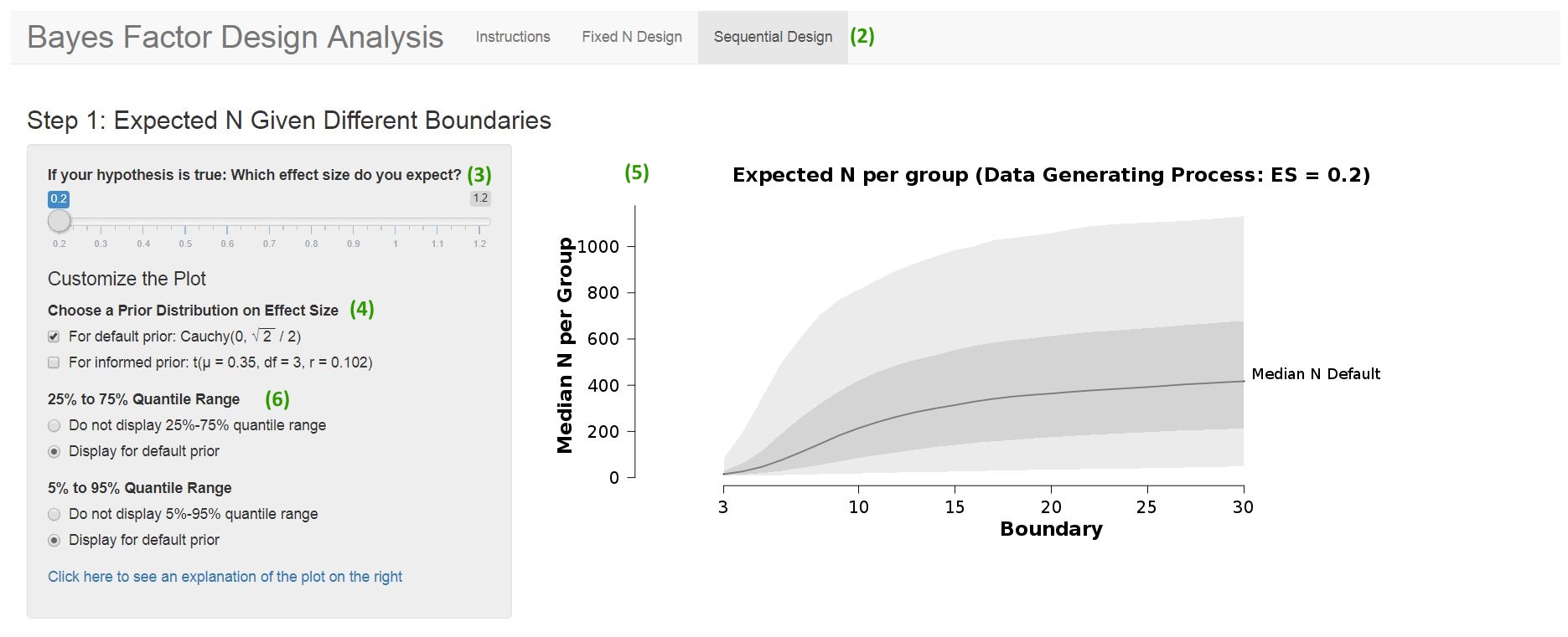
Figure 2: Screenshot from the BFDA App. Get an overview on expected sample sizes in sequential Bayesian designs.
- Open the BFDA App (http://shinyapps.org/apps/BFDA/) in a web browser. Depending of the number of users, this may take a minute, but while you are waiting you can already ponder the definition of your research design (step 2-4).
- Choose a design: Here we focus on sequential designs, so select the “Sequential Design” tab. The user interface should now look like Figure 2.
- Choose a data-generating effect size under H1: This defines the population from which you want to draw samples. You can either choose the effect size you expect when your hypothesis is true, or choose an effect size that is somewhat smaller than you expect (following a safeguard power approach, Perugini et al. 2014), or a smallest effect size of interest (SESOI). For this example, we choose an effect size of = 0.2and assume that this is your SESOI. You can choose this effect size on the slider in the top part of the app.
- Choose a prior distribution on effect size that will be used for the analysis: Say, you do not have much prior information. You only know that under your alternative hypothesis group A should have a larger mean than group B. With this information, it is reasonable to choose a “default” prior on effect size. You can do this by ticking the “For default prior” box in the top left panel of the app.
- These options yield an overview plot in the top right of the app. The plot displays the expected (median) sample sizes per group depending on the chosen evidence boundaries. Remember: These boundaries are the evidence thresholds, that is, the Bayes factor values at which you stop collecting data. Unsurprisingly, larger sample sizes are required to reach higher evidence thresholds. You can use this plot to find a good balance between expected sample sizes (“study costs”) and obtained evidence (“study benefits”).
- If you want to get an impression of the whole distribution of sample size for all boundaries, you can tick the “Quantile” options on the left to see the 25% and 75% and/or the 5% and 95% quantile of the distributions in the plot. Unsure how to interpret this? Click on the “Click here to see an explanation” button, and you will see an explanation.
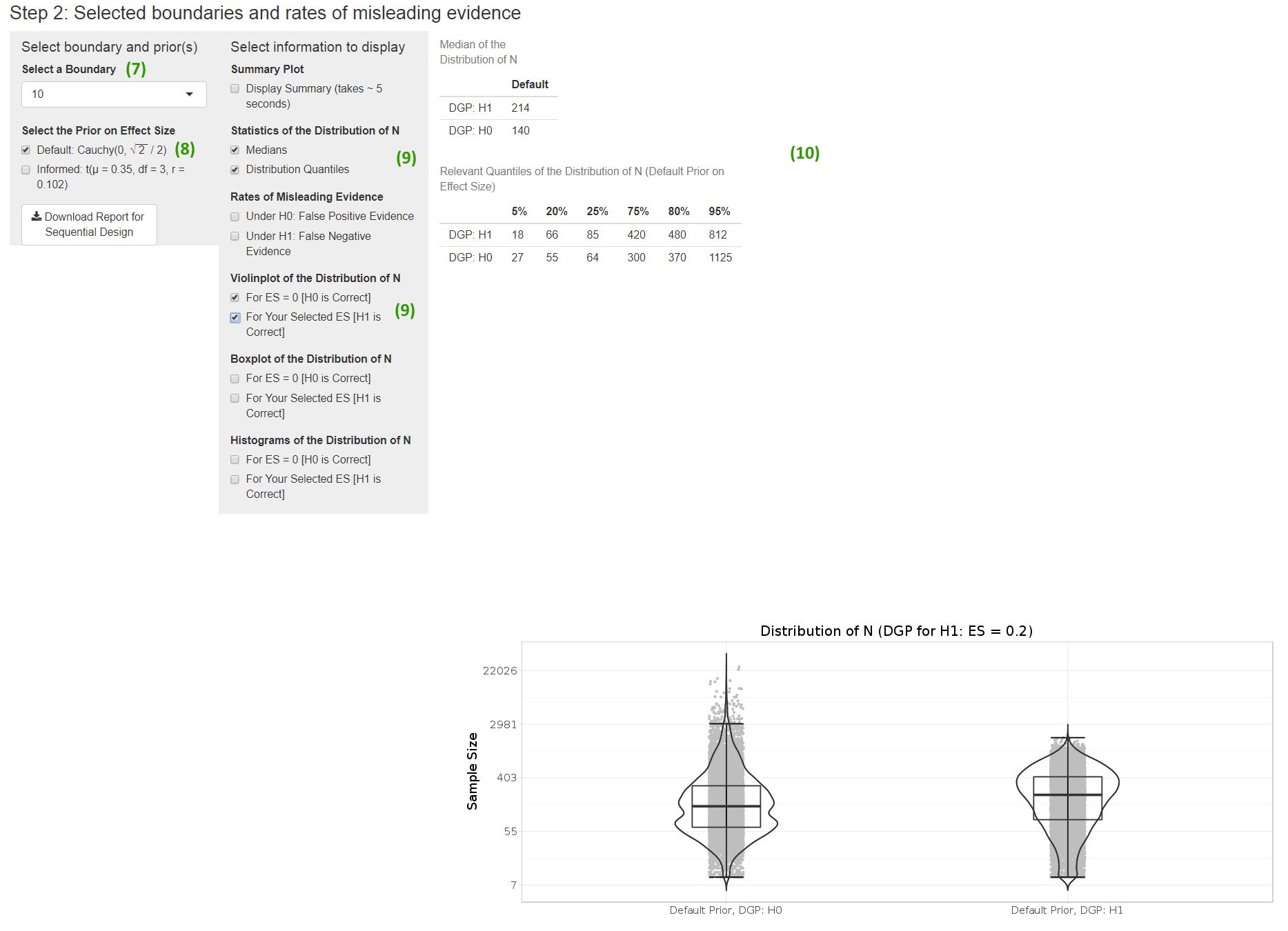
Figure 3: Screenshot from the BFDA App. Investigate sample size distributions and rates of misleading evidence for different boundaries in sequential designs.
After inspecting the overview plot, you can continue with step 2 in the app (displayed in Figure 3).
- Select a boundary: Say you want to obtain “strong evidence”, meaning a Bayes factor of 10 or smaller than 1/10 (Lee & Wagenmakers, 2013, p. 105), so you select a boundary of 10 in the drop-down menu.
- Select the prior distribution: We had selected the default prior above, so it is reasonable to do the same here.
- Select the information that should be displayed: For this example, we select both numeric (medians, distribution quantiles) and pictorial representations (a violin plot) from the list.
- The results of the Monte Carlo simulation are displayed on the right. They include both the results under your alternative hypothesis ( = 0.2) and under the null hypothesis ( = 0). The expected (median) sample size is 214 under the alternative hypothesis (H1) and 140 under the null hypothesis (H0). If you need to provide an upper boundary on required sample sizes (for example, if you are applying for grant money), we would recommend using the larger 80% quantile (in this case 480 observations per group).
Now you have arrived at your destination. You know how many participants you can expect to test in order to obtain strong evidence. You can summarize the results from the App in a proposal for a registered report; if you want to be extra-awesome you can use the App to download a time-stamped report (click on the “Download Report for Sequential Design” button) and attach it to your submission. This was easy, wasn’t it?
Want to know more?
Excited about the opportunities of Bayes Factor Design Analysis? Check out our recent PsyArXiv preprint for more information.
I want to thank Felix Schönbrodt, Quentin Gronau, and Eric-Jan Wagenmakers for their advice on the project and for their comments on earlier versions of this blog post.
Like this post?
Subscribe to the JASP newsletter to receive regular updates about JASP including the latest Bayesian Spectacles blog posts! You can unsubscribe at any time.
References
Gronau, Q. F., Ly, A., & Wagenmakers, E.-J. (2017). Informed Bayesian t-tests. arXiv preprint. Retrieved from https://arxiv.org/abs/1704.02479
Lee, M. D. & Wagenmakers, E.-J. (2014) Bayesian cognitive modeling: A practical course. Cambridge University Press.
Morey, R., & Rouder, J. N. (2015). BayesFactor: Computation of Bayes factors for common designs. Retrieved from https://cran.r-project.org/web/packages/BayesFactor/index.html
Perugini, M., Gallucci, M., & Costantini, G. (2014). Safeguard power as a protection against imprecise power estimates. Perspectives on Psychological Science, 9(3), 319–332. doi: 10.1177/ 1745691614528519 664
Rouder, J. N. (2014). Optional stopping: No problem for Bayesians. Psychonomic Bulletin & Review, 21(2), 301-308. doi: 10.3758/s13423-014-0595-4
Schönbrodt, F. D., & Wagenmakers, E.-J. (in press). Bayes factor design analysis: Planning for compelling evidence. Psychonomic Bulletin & Review. doi: 10.3758/s13423-017-1230-y
Schönbrodt, F. D., Wagenmakers, E.-J., Zehetleitner, M., & Perugini, M. (2017). Sequential hypothesis testing with Bayes factors: Efficiently testing mean differences. Psychological Methods, 22(2), 322–339. doi: 10.1037/met0000061
Wagenmakers, E. J., Morey, R. D., & Lee, M. D. (2016). Bayesian benefits for the pragmatic researcher. Current Directions in Psychological Science, 25(3), 169-176. doi: 10.1177/0963721416643289
Wald, A. (1945). Sequential tests of statistical hypotheses. The Annals of Mathematical Statistics, 16(2), 117-186. doi: 10.1214/aoms/1177731118
About The Author

Angelika Stefan
Angelika is a psychology master student at LMU Munich and does a research internship at the Psychological Methods Group at the University of Amsterdam.