What Determines the Price of LEGO Sets? A Bayesian Analysis with Twists and Turns

July 10 - 2023

Recently we completed a multi-year Odyssey in order to obtain Bayes factors for partial correlations. The result is now available as a preprint.

Instead of delving into the finer details of Bayes factors and posterior distributions, we will provide a concrete demonstration. Specifically, we will use Bayes factors for partial correlations to address a perennial question that has tormented children and parents alike: what determines the price of LEGO sets? Of course this important question has been studied previously (e.g., Peterson & Ziegler, 2021 – hat tip to Quentin Gronau), and here our purpose is merely to demonstrate how a statistical association between two variables can flip from positive to negative to neutral, depending on what other variables are taking into consideration. Get ready: you are in for a bumpy ride.

A Positive Association!

We start by opening the LEGO data set: https://osf.io/e9yh6 (i.e., the data set provided by Peterson and Ziegler, with entries removed that have missing values) which contains prices for 265 different LEGO sets. For each set there are several variables. We are interested in whether “Price” is associated with “Minimum Age” (i.e., the age that is shown on the box). In a first analysis, we consider the scatter plot between the two variables. Of course we use JASP throughout. Here is the result:

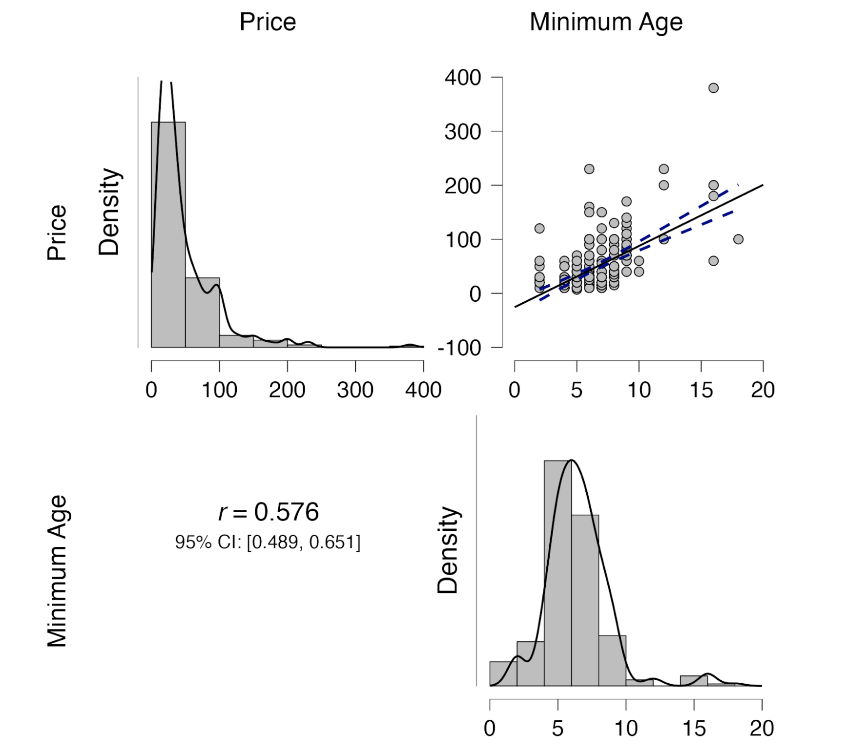
It appears that we can be relatively certain that the price of LEGO increases when the age indicated on the box is higher. In terms of a statistical significance test, the p-value for the two-sided test equals $8\times10^{-25}$, which is rather small. But as low as that p-value may be, it does not tell us whether the data were less likely under H0 than under H1; in other words, we do not actually know whether and to what extent the data undercut or support H0.

So we turn to a default Bayesian analysis for correlations. With a few mouse clicks in JASP we learn that the Bayes factor in favor of H1 over H0 equals $5.26\times10^{21}$: truly astronomical evidence against H0 (versus the default specification of H1). In this case, misinterpreting the p-values in terms of statistical evidence would not have led you astray.

A Negative Association!
But we can dig a little deeper. We know that sets for older kids (or adults) generally have more pieces, so it is no wonder that those sets are more expensive. What if we “control for” or “partial out” the effect of the number of pieces? Will there still be a positive association between Price and Minimum Age? We return to a frequentist analysis and execute the partial correlation analysis. Somewhat surprisingly perhaps, we find that the partial correlation coefficient between Price and Minimum Age has flipped sign and is now negative: partial r = -0.31, 95%CI=[-0.55,-0.08], with an associated p-value of $3.26\times10^{-7}$, which is still very low (i.e., p = 0.00000032597).

In order to ascertain how much evidence this is against H0, we would ideally conduct a Bayesian test for a partial correlation. This test is not (yet!) implemented in JASP, but the Kucharsky preprint allows us to obtain the answer: the Bayes factor for the default specification of H1 over H0 equals $32.71\times10^{3}$. Again, a misinterpretation of the p-value in terms of something that addresses a meaningful question would not have led you astray.

No Association?!
The above analysis suggests that, correcting for the number of blocks, LEGO sets are more expensive for younger kids than for older kids. This could be the result of some devious LEGO marketing strategy, where parents are (rightly) assumed to willingly overpay in order to safeguard the satisfaction of their offspring. Alternatively, it may just be that the LEGO blocks are larger when they are part of sets meant for younger kids. Consequently, we wish to learn about the association between Price and Minimum Age while “controlling” or partialling out both the effect of number of pieces and the effect of the weight of the sets. We first turn to the frequentist analysis, and find that the partial correlation between Price and Minimum Age is now much reduced: partial r = 0.09, 95%CI=[-0.21,0.35], with an associated p-value of 0.15. So the partial correlation is no longer “statistically significant”. But is there absence of evidence or evidence of absence? (e.g., Keysers et al., 2020). In order to find out, we resort again to the methodology outlined in the Kucharsky preprint, and find that a default test for partial correlations yields BF10 = 0.22; in other words, the data are about 1/0.22 = 4.55 more likely under H0 than under H1; this is moderate support for H0.

Full Data Set: The Plot Thickens

The previous analyses were conducted on a subset of 265 LEGO sets, because we removed all sets with missing values. However, when we focus solely on the variables of interest, there are many more complete entries. Repeating the analysis on this “full” data set generally yields the same pattern of results. However, we find something mysterious as well. The full data set is available at https://osf.io/9h54c.

For the full data set (N = 1042 complete entries), the correlation between Price and Minimum Age equals r = 0.56, 95%CI = [0.52, 0.60], $p = 1.14\times10^{-87}$. With the number of pieces partialled out (still N = 1042 complete entries), we have r = -0.15, 95%CI = [-0.25, -0.05], $p = 1.37 \times 10^{-6}$. The interesting result occurs when both number of pieces and weight are partialled out (now N = 404 complete entries). That gives the following result: r = 0.15, 95%CI = [-0.08, 0.32], $p = .0035$. First, note that adding the weight variable results in a much higher p-value, even though the absolute value of the sample correlation is about the same; this can be explained because the weight variable is often missing from the data set, such that the sample size for the two analyses is very different. Second, note that in the final analysis, the p-value is .0035 even though the 95% CI contains zero. This contradiction occurs because the confidence intervals for partial correlations are obtained from the bootstrap. The fact that the bootstrap interval is at odds with the p-value suggests that the model may be misspecified and perhaps contain outliers (a quick Google search came up short – please email us if you know more about this phenomenon).

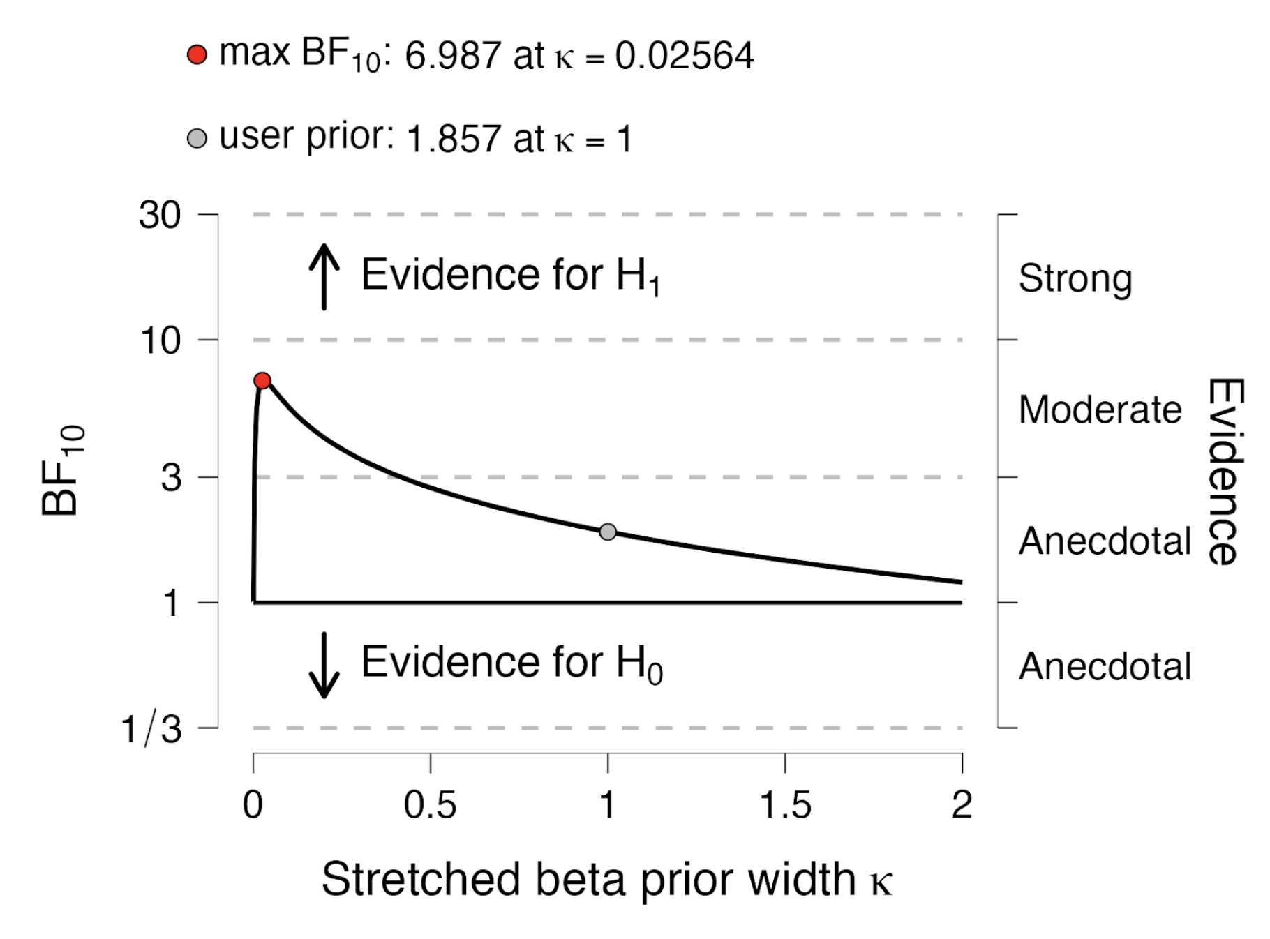
To examine this possibility we compute Spearman’s rho, a metric that takes only rank information into account. When we do this we encounter a final surprise: for Spearman’s rho, we have that r = -0.13, 95%CI = [-0.25, -0.013], $p = .0091$. The association is negative once more! What to believe? The Kucharsky preprint allows us to compute a Bayesian partial Spearman’s rho (obtained by first transforming the variables to ranks, and then applying Pearson’s analysis). When we do this, we find that the Bayes factor equals BF10=1.86, meaning that the data are about 1.86 more likely under H1 than under H0; this is anecdotal evidence for H1. The figure below shows that when the width of the prior distribution for the partial correlation coefficient is changed, the evidence fluctuates from about 7 to 1; it seems premature to draw strong conclusions (such as “reject the null hypothesis”) based on such a result.

Into the Rabbit Hole

As an aside, an inspection of the scatter plots in the first figure suggests that both price and pieces may need to be log-transformed. For the log-transformed variables, the partial correlation between LogPrice and Minimum Age (with LogPieces partialled out) is no longer negative: r = 0.045, 95%CI = [-0.09, 0.15], $p = .15$. But when we then partial out weight as well, we find that the partial correlation, instead of being absent, is negative (as it was for Spearman’s rho): r = -0.27, 95%CI = [-0.42, -0.14], $p = 5.90 \times 10^{-8}$.

And now for our final twist. What we have not done is log transform the weight variable. When we do this and compute the partial correlation between LogPrice and Minimum Age (with LogPieces and LogWeight partialled out) we find that the association is again positive: r = 0.23, 95%CI = [0.04, 0.36], $p = 3.78 \times 10^{-6}$.

It is remarkable that a seemingly straightforward analysis with only four variables can produce so many surprises. Depending on what variables are partialled out and/or transformed, the association between price and age is either negative, positive, or absent. We suspect that we have scratched only the surface here, and we may return to the topic in a later post.

When we searched for information on this flip-flopping of the partial correlation coefficient, we landed on an online discussion: https://stats.stackexchange.com/questions/1580/regression-coefficients-that-flip-sign-after-including-other-predictors with a few relevant articles (e.g., Knaeble & Dutter, 2015; Onyebuchi, 2008; Tu et al., 2008).

References

Onyebuchi, A. A. (2008). The role of causal reasoning in understanding Simpson’s paradox, Lord’s paradox, and the suppression effect: covariate selection in the analysis of observational studies. Emerging Themes in Epidemiology, 5:5. URL: https://ete-online.biomedcentral.com/articles/10.1186/1742-7622-5-5

Keysers, C., Gazzola, V., & Wagenmakers, E.-J. (2020). Using Bayes factor hypothesis testing in neuroscience to establish evidence of absence. Nature Neuroscience, 23, 788-799. URL: https://pure.uva.nl/ws/files/52486656/s41593_020_0660_4.pdf

Knaeble, B., & Dutter, S. (2015). Reversals of least-squares estimates and model-independent estimation for directions of unique effects. URL: https://arxiv.org/abs/1503.02722

Kucharský, Š., Wagenmakers, E.-J., van den Bergh, D., & Ly, A. (2023). Analytic posterior distribution and Bayes factor for Pearson partial correlations. Manuscript submitted for publication. URL: https://psyarxiv.com/6muwy/

Peterson, A. D., & Ziegler, L. (2021). Building a multiple linear regression model with LEGO brick data. Journal of Statistics and Data Science Education, 29, 297-303.

The LEGO data used in the above analyses can be found at https://osf.io/e9yh6 (NAs removed) and at https://osf.io/9h54c (NAs retained).

Tu, Y-K., Gunnell, D., & Gilthorpe, M. S. (2008) Simpson’s Paradox, Lord’s Paradox, and Suppression Effects are the same phenomenon – the reversal paradox. Emerging Themes in Epidemiology, 5:2. URL: https://ete-online.biomedcentral.com/articles/10.1186/1742-7622-5-2