Order-restrictions in JAGS: Five Methods Fail, One Method Succeeds

July 24 - 2023

TL;DR When implementing order-restrictions in JAGS, only the “ones trick” appears to yield the correct result.

Consider two unknown chances, $\theta_1$ and $\theta_2$, that are assigned independent beta priors: $\theta_1 \sim \text{beta}(1,1)$ and $\theta_2 \sim \text{beta}(1,1)$. Let’s visualize the joint posterior by executing JAGS code (Plummer, 2003) and plotting the samples that are obtained from the MCMC algorithm. This is easy to accomplish in JASP, which boasts a recently revamped “JAGS module”. Open JASP, activate the “JAGS” module from the module list, and enter the following JAGS syntax:

model{
theta1 ~ dbeta(1,1)
theta2 ~ dbeta(1,1)
}

We also indicate that “theta1” and “theta2” are the parameters we wish to monitor. Pressing “control+enter” then runs the JAGS model and returns samples from the two chances. We go to “plots” and tick “bivariate scatter”, and select the “contour” option. This is the result:

The off-diagonal contour plot confirms that the joint posterior is relatively flat. So far so good.

However, now we wish to add to this prior specification the restriction that $\theta_1 > \theta_2$. As noted in O’Hagan & Forster (2004, pp. 70-71), this restriction represents additional information, and as such it can be entered at any stage of the Bayesian learning process. We could for instance add the restriction at the end and simply remove all the MCMC samples that violate the restriction. If we were to do this, the joint distribution would still be uniform but only occupy half of the area it did previously. However, the procedure of eliminating samples becomes increasingly inefficient as the restriction becomes more specific. It would therefore be worthwhile to consider adding the restriction at the very beginning, by adjusting the prior. As it turns out, this is surprisingly difficult to accomplish.

It is clear what the end result should be: a flat joint distribution that has mass only in the region consistent with the restriction. First we’ll show five beguiling procedures that fail to do the job. Some of these procedures are from highly reputable sources and as a result have become the norm.

Fail 1
model{
theta1 ~ dunif(0,1)
theta2 ~ dunif(0,theta1)
}

This yields the following scatter plot:

Whoops! This is not what we would like to see. Let’s try something else.

Fail 2
model{
theta1 ~ dbeta(1,1)
theta2 ~ dbeta(1,1)I(,theta1)
}

This gives the same undesirable result:

Bummer. Another attempt then.

Fail 3
model{
theta1 ~ dunif(0,1)
p ~ dunif(0,1)
theta2 <- p*theta1
}

No cigar. Let’s try some other ideas:

Fail 4
model{
theta1 ~ unif(0,1)I(theta2,1)
theta2 ~ unif(0,1)I(0,theta1)
}

This trick was proposed by a friend of a friend. Unfortunately, it returns the error message “possible directed cycle” (JAGS models must be directed acyclic graphs). Moving on…

Fail 5
model{
thetap[1] ~ dbeta(1,1)
thetap[2] ~ dbeta(1,1)
thetaprior[1:2] <- sort(thetap[])
theta2 <- thetaprior[1] theta1 <- thetaprior[2] }

This is more or less the officially sanctioned version, and at first glance it does appear to work:

The contour plots indicate a flat joint posterior. Hurray! The marginal distributions are not uniform but that is the correct result (e.g., $\theta_2$ has predominantly low values, since the higher values run an increasing risk of being truncated).

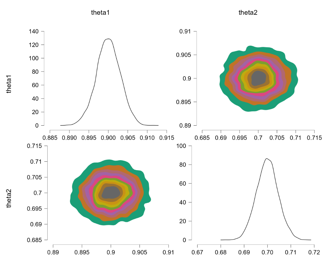
Before popping the champagne bottle it pays to consider what the sort-solution really does. Essentially it samples from the joint distribution and when a pair of theta’s violate the restriction they are switched, that is, the values are reflected along the main diagonal. For instance, a violation of $\theta_1 = 0.4, \theta_2 = 0.6$ would be changed to $\theta_1 = 0.6, \theta_2 = 0.4$, which falls in the allowed parameter region. Reflecting the values that violate the restriction is fundamentally different from eliminating them (and then renormalizing), at least for distributions that are asymmetric about the main diagonal. To illustrate, consider the following distributions: $\theta_1 \sim \text{beta}(7000,3000)$ (a distribution highly peaked around .70) and $\theta_2 \sim \text{beta}(9000,1000)$ (a distribution highly peaked around .90). Imposing the restriction that $\theta_1 > \theta_2$ by means of the code above yields the following outcome:

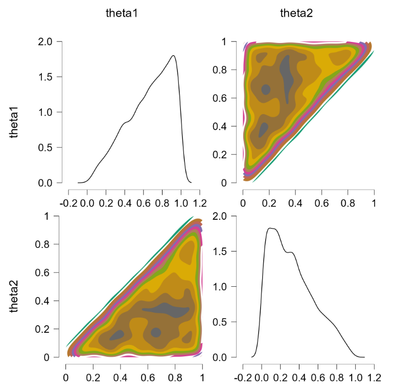
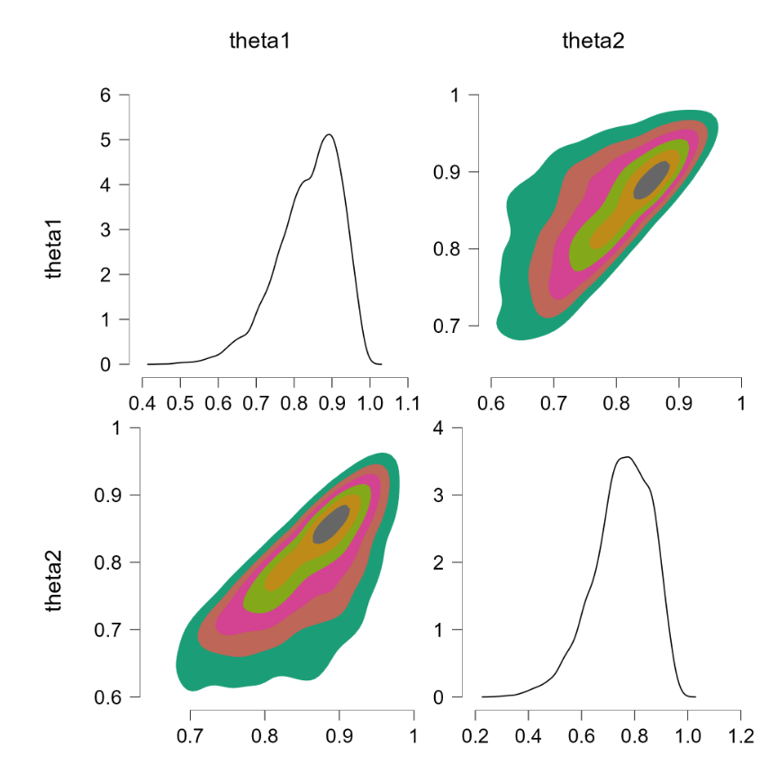
The “sort” trick has essentially flipped the prior distributions: $\theta_1$ is now centered around .90 (instead of around .70) and $\theta_2$ is now centered around .70 (instead of around .90). But this method of imposing an order-restriction is not correct – truncating the unrestricted joint distribution and renormalizing would not result in such a flip. Let’s consider a restriction that is less extreme, based on $\theta_1 \sim \text{beta}(7,3)$ and $\theta_2 \sim \text{beta}(9,1)$. The code above produces the following result:

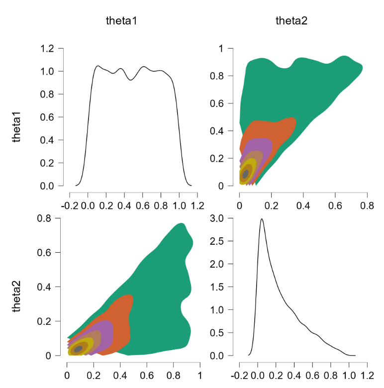
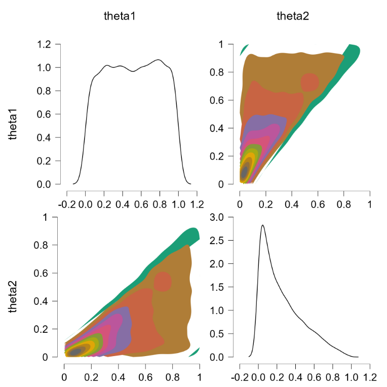
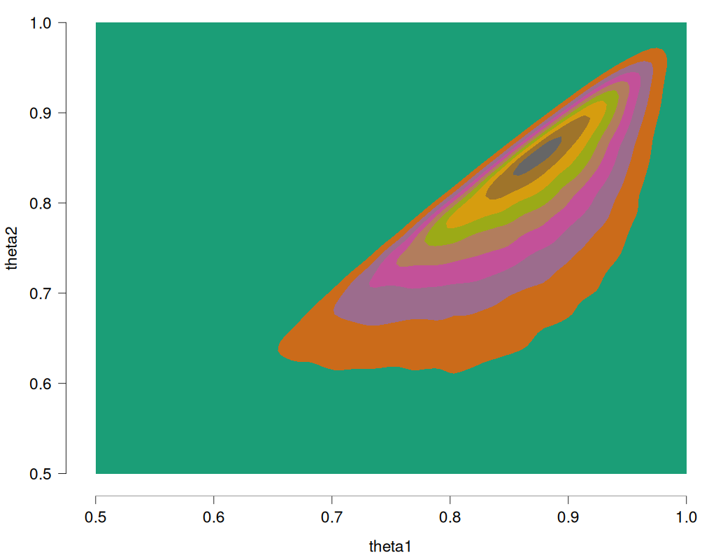
As before, the sort trick has essentially reversed the roles of the priors. Note again that this is different from the solution we know to be correct, namely to obtain the joint distribution without the restriction, and then truncating and renormalizing the joint distribution. For reference, this is what the restricted joint distribution should be (obtained from rejection sampling, R code at the end of this post):

Finally: Success with the “Ones Trick”!

The following code is based on the “ones trick” and it is the only solution that worked, at least when some remaining hurdles are cleared. However, we again start with another failure, for good measure. Specifically, this code does not work:

model{
theta1 ~ dbeta(1,1)
theta2 ~ dbeta(1,1)
z <- 1
z ~ dbern(constraint)
constraint <- step(theta1-theta2)
}

In JAGS this returns an error: “attempt to redefine node z[1]”

Fortunately, the solution does work when z <- 1 is passed as data:

data{
z <- 1
}

model{
theta1 ~ dbeta(1,1)
theta2 ~ dbeta(1,1)
z ~ dbern(constraint)
constraint <- step(theta1-theta2)
}

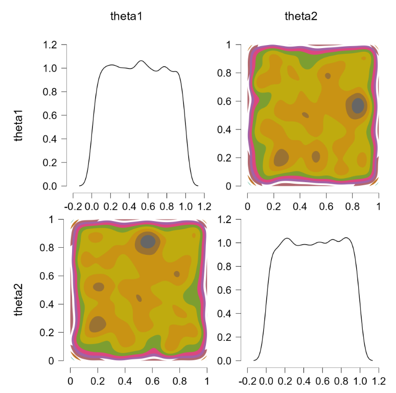
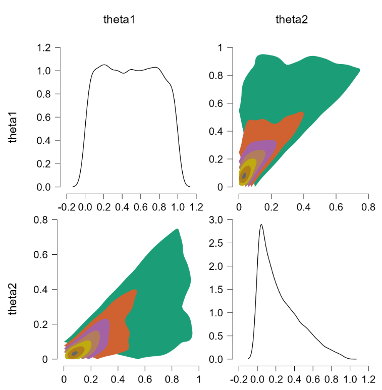
Applying this code yields the following outcome:

Finally, the joint distribution is uniform. We now consider the example discussed earlier, where $\theta_1 \sim \text{beta}(7,3)$ and $\theta_2 \sim \text{beta}(9,1)$. Alas, this code also returns an error:

data{
z <- 1
}

model{
theta1 ~ dbeta(7,3)
theta2 ~ dbeta(9,1)
z ~ dbern(constraint)
constraint <- step(theta1-theta2)
}

The error is “node inconsistent with parents”. This suggests that we select initial values for theta1 and theta2 that adhere to the restriction. In JASP we can do so under the tab “Initial Values”. When we assign initial values of, say, 0.8 to theta1 and 0.7 to theta2, we obtain the following result:

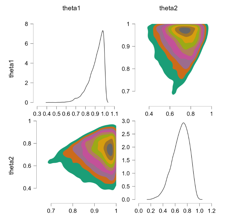
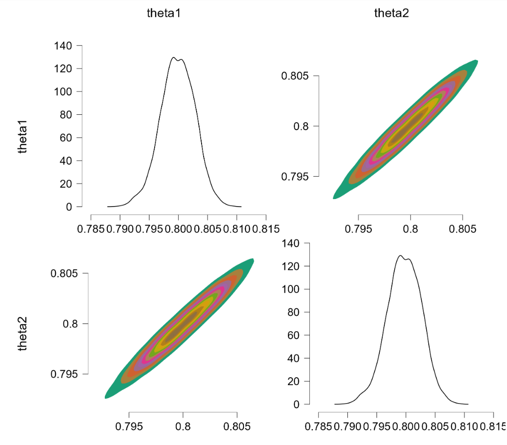
This is promising. We now turn to the more challenging problem where $\theta_1 \sim \text{beta}(7000,3000)$ and $\theta_2 \sim \text{beta}(9000,1000)$. The restriction is extreme and in order to obtain sufficient samples from the truncated prior we thin by 100, use 2,000 samples burnin, and draw 200,000 samples. The results:

Conclusion

It is often said that with the help of MCMC, the specification of a model is limited only by the user’s imagination. This is true, but the flip side of this flexibility is that the number of ways a model can be implemented incorrectly is also limited only by the user’s imagination. In this post we have shown six ways to implement a simple order-restriction for two binomial chances. Several of these were beguiling, but only a single method –the `ones’ trick with the proper initial assignment– was correct.

Appendix: Rejection Sampling R Code for the Restricted Beta Distribution

library(jaspGraphs) # install via remotes::install_github(“jasp-stats/jaspGraphs”)
library(ggplot2)
n <- 1e6
x1 <- rbeta(n, 7, 3)
x2 <- rbeta(n, 9, 1)
idx <- which(x1 > x2)
df <- data.frame(x = x1[idx], y = x2[idx])
ggplot(data = df, aes(x, y)) +
geom_density_2d_filled() +
scale_x_continuous(name = “theta1”, limits = c(.5, 1)) +
scale_y_continuous(name = “theta2”, limits = c(.5, 1)) +
jaspGraphs::scale_JASPfill_discrete() +
jaspGraphs::geom_rangeframe() +
jaspGraphs::themeJaspRaw()

References

O’Hagan, A., & Forster, J. (2004). Kendall’s advanced theory of statistics vol. 2B: Bayesian inference (2nd ed.). London: Arnold.

Plummer, M. (2003). JAGS: A program for analysis of Bayesian graphical models using Gibbs sampling. In Hornik, K., Leisch, F., & Zeileis, A. (Eds.), Proceedings of the 3rd International Workshop on Distributed Statistical Computing. Vienna, Austria.