My colleague Raoul Grasman and I recently posted the preprint “A discrepancy measure based on expected posterior probability“. In this preprint, we show that the expected posterior probability for a true model Hf equals the expected posterior probability for a true alternative model Hg. It is not immediately obvious why this should be the case. In Appendix A of the preprint, we provide a geometric interpretation of this result, and I will present that interpretation in this blogpost as well.
Geometric Intuition
Assume that future data x will be drawn either from f(x), the prior predictive distribution for model Mf, or from from g(x), the prior predictive distribution for rival model Mg. We assume that both models are equally likely a priori. The key result is that the expected posterior probability for a true Mf equals that of a true Mg, that is, E[p(Mf | xf)] = E[p(Mg | xg)]. To intuit why this should be the case, consider the figure below:
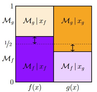
On the x-axis, there are two possibilities, namely that the observation x will be drawn from f(x) or from g(x); when we assume that the data-generating models Mf and Mg are equally likely, f(x) and g(x) each occupy half of the x-axis domain. The y-axis shows the posterior probability for Mf versus Mg. In the figure, the expected posterior probability for a true Mf equals 0.60 (i.e., the deep purple square: E[p(Mf | xf)]). This has two immediate and inevitable consequences. First, the complement of this probability (i.e., 1-0.60 = 0.40) is E[p(Mg | xf)]), the posterior probability for the rival hypothesis Mg expected under f(x) (i.e., the light yellow square). At the same time, however, the fact that the expected posterior probability for Mf equals its prior probability (e.g., Goldstein, 1983) implies that whatever Mf gains in expectation under f(x), it should lose again under g(x). Visually, this means that the expected gain in credibility for Mf when it is true (i.e., 0.60 – 0.50, as indicated by the double arrows in the deep purple square) needs to equal the expected loss in credibility for Mf when it is false (i.e., 0.50 – 0.40, as indicated by the double arrows in the deep yellow square). This then leaves an expected posterior probability of 0.60 for a true Mg. Essentially, E[p(Mg | xg)] equals E[p(Mf | xf)] because it is the complement of its complement.
Paradox?
As the preprint mentions, it is well-known that under default prior distributions, the expected Bayes factors in favor of a true H1 increase much faster than those for a true H0. It is way easier to find evidence for the existence of an effect than for its absence. This makes intuitive sense: if you did find an effect, it is clear that H0 cannot account for it; but if you have not found an effect, you may still be doubtful whether it is truly null or just very small — H1 can account for small effects, so the only way that H0 can beat H1 is through parsimony. This means that on the level of Bayes factors, it is difficult for H0 to come out on top. At the same time, however, the expected posterior probability in favor of a true H1 equals exactly that for a true H0. So on the level of posterior probabilities, the evidential assymmetry disappears completely. Both are facts of probability theory, both can be grasped intuitively, but it is challenging to accept them at the same time.
Preprint Abstract
“Two prior predictive distributions f(x) and g(x) are associated with two equally plausible models Mf and Mg, respectively. A single observation x would update the probability of Mf from 1/2 to f(x) /[f(x) + g(x)]. The discrepancy D_EP(f || g) between distributions f(x) and g(x) equals E[p(Mf|xf)], that is, the expected posterior probability for Mf after a single observation x from f(x). In contrast to the Kullback-Leibler discrepancy (which is based on the expected logarithm of the Bayes factor for Mf) the discrepancy D_EP(f || g) (a) is symmetric in the sense that D_EP(f || g) = D_EP(g || f); (b) is defined even when the two distributions are not absolutely continuous with respect to one another; (c) is robust to differences in the tail of the distributions; and (d) quantifies dissimilarity of distributions on the familiar scale of probability. For hypothesis testing, this implies that the expected posterior probability for a true null hypothesis H0 equals the expected posterior probability for a true alternative hypothesis H1, despite the fact that default Bayes factors generally accumulate much more quickly for a true H1 than they do for a true H0.”
References
Goldstein, M. (1983). The prevision of a prevision. Journal of the American Statistical Association, 78, 817–819.
Wagenmakers, E.-J. & Grasman, R. P. P. P. (2025). A discrepancy measure based on expected posterior probability. Manuscript submitted for publication.